Cutaneous melanoma (SKCM) is the most invasive malignancy of skin cancer. Metastasis to distant lymph nodes or other system is an indicator of poor prognosis in melanoma patients. The aim of this study was to identify reliable prognostic biomarkers for SKCMs.
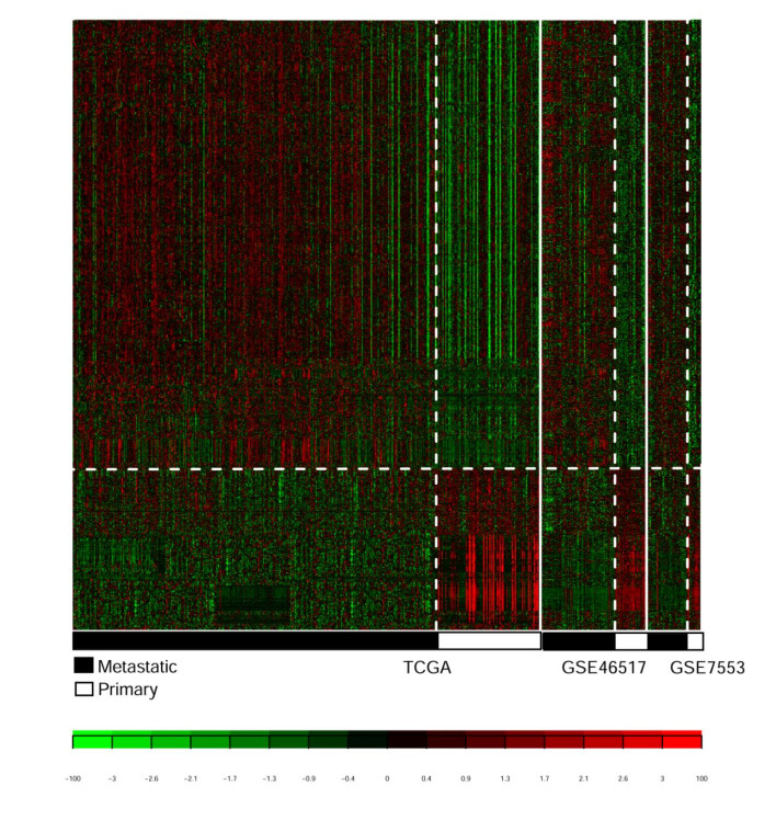
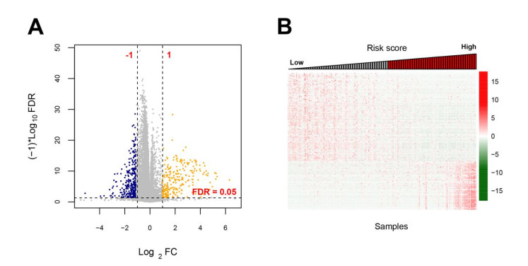
Four RNA-sequencing datasets associated with SKCMs were downloaded from the Gene Expression Omnibus (GEO) and The Cancer Genome Atlas (TCGA) database as well as corresponding clinical information. Differentially expressed genes (DEGs) were screened between primary and metastatic samples by using MetaDE tool. Weighted gene co-expression network analysis (WGCNA) was conducted to screen functional modules. A prognostic score (PS)-based predictive model and nomogram model were constructed to identify signature genes and independent clinicopathologic factors.
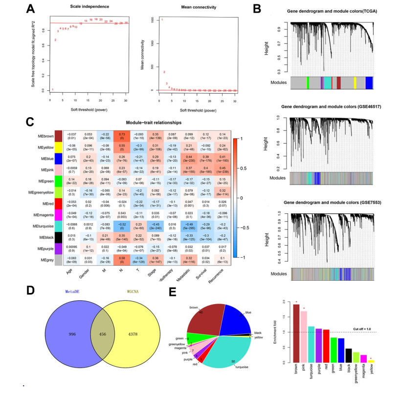
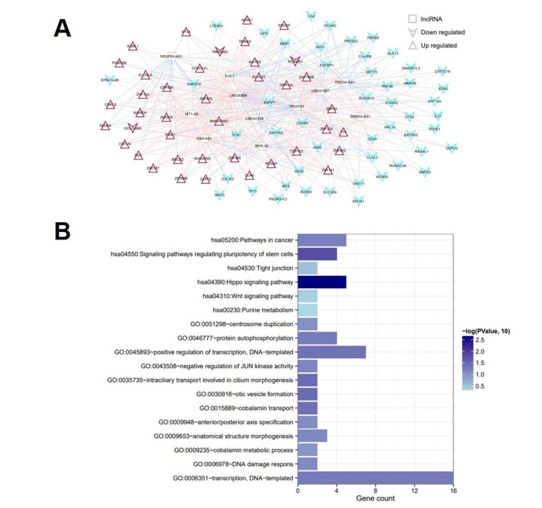
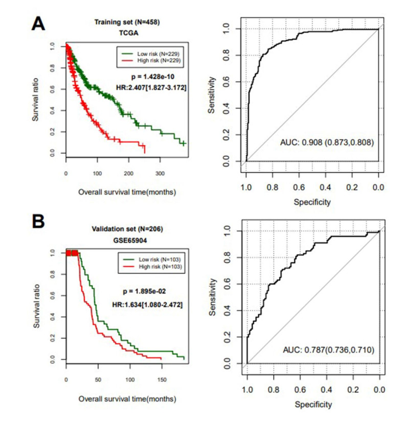
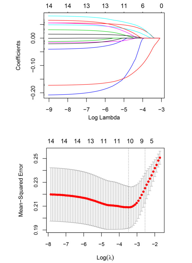
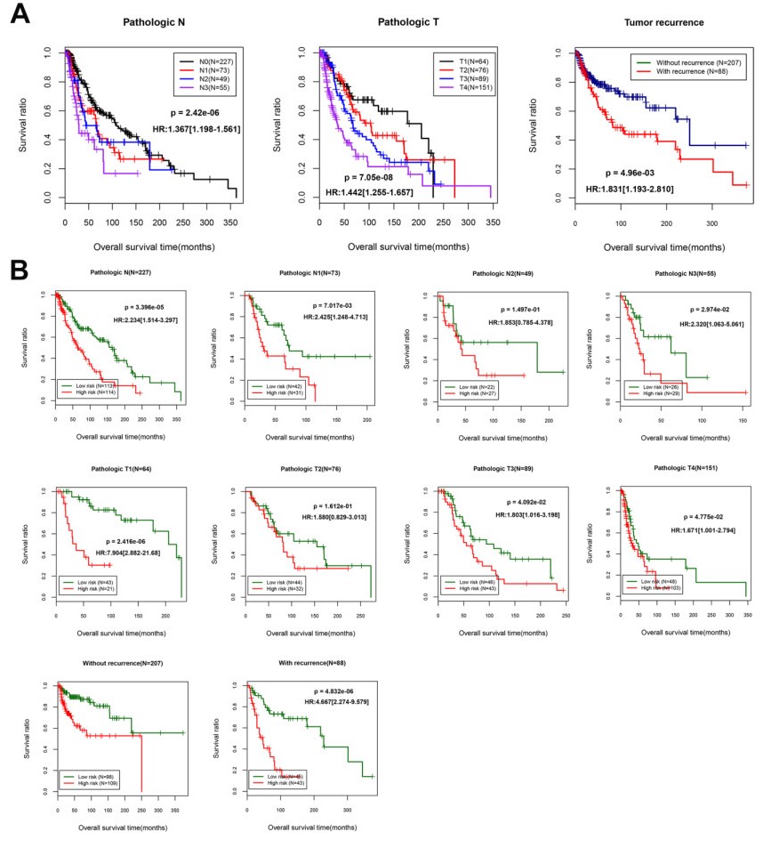
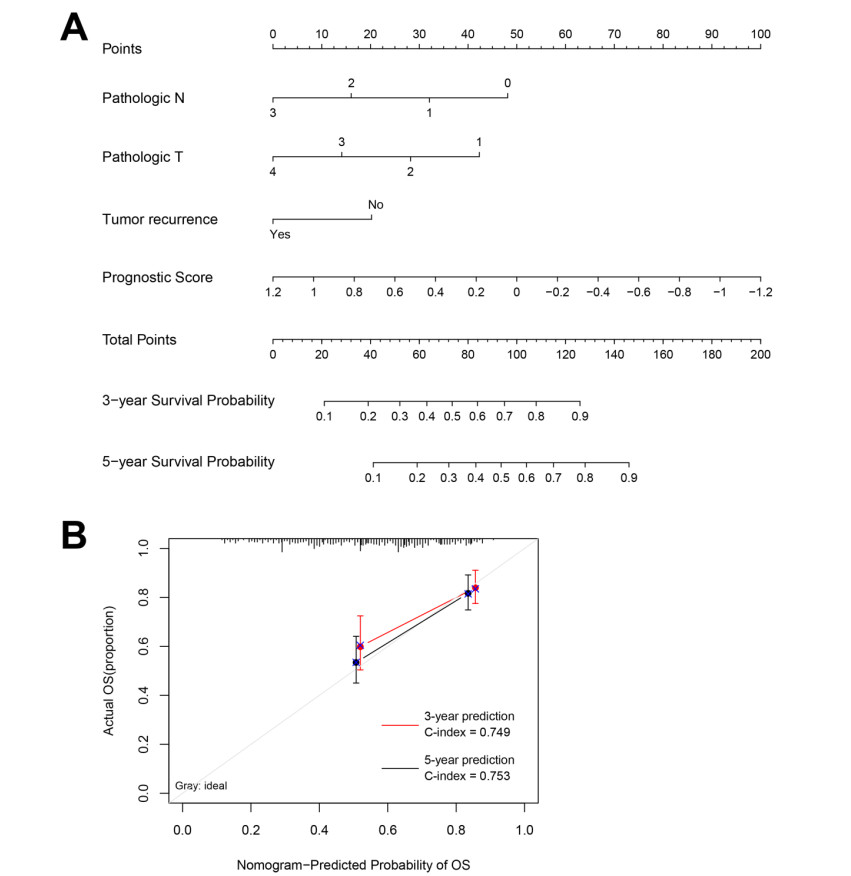
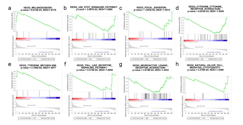
Based on MetaDE analysis and WGCNA, a total of 456 overlapped genes were identified as hub genes related to SKCMs progression. Functional enrichment analysis revealed these genes were mainly involved in the hippo signaling pathway, signaling pathways regulating pluripotency of stem cells, pathways in cancer. In addition, eight optimal DEGs (RFPL1S, CTSV, EGLN3, etc.) were identified as signature genes by using PS model. Cox regression analysis revealed that pathologic stage T, N and recurrence were independent prognostic factors. Three clinical factors and PS status were incorporated to construct a nomogram predictive model for estimating the three years and five-year survival probability of individuals.
The prognosis prediction model of this study may provide a promising method for decision making in clinic and prognosis predicting of SKCM patients.
Citation: Jiaping Wang. Prognostic score model-based signature genes for predicting the prognosis of metastatic skin cutaneous melanoma[J]. Mathematical Biosciences and Engineering, 2021, 18(5): 5125-5145. doi: 10.3934/mbe.2021261
Cutaneous melanoma (SKCM) is the most invasive malignancy of skin cancer. Metastasis to distant lymph nodes or other system is an indicator of poor prognosis in melanoma patients. The aim of this study was to identify reliable prognostic biomarkers for SKCMs.
Four RNA-sequencing datasets associated with SKCMs were downloaded from the Gene Expression Omnibus (GEO) and The Cancer Genome Atlas (TCGA) database as well as corresponding clinical information. Differentially expressed genes (DEGs) were screened between primary and metastatic samples by using MetaDE tool. Weighted gene co-expression network analysis (WGCNA) was conducted to screen functional modules. A prognostic score (PS)-based predictive model and nomogram model were constructed to identify signature genes and independent clinicopathologic factors.
Based on MetaDE analysis and WGCNA, a total of 456 overlapped genes were identified as hub genes related to SKCMs progression. Functional enrichment analysis revealed these genes were mainly involved in the hippo signaling pathway, signaling pathways regulating pluripotency of stem cells, pathways in cancer. In addition, eight optimal DEGs (RFPL1S, CTSV, EGLN3, etc.) were identified as signature genes by using PS model. Cox regression analysis revealed that pathologic stage T, N and recurrence were independent prognostic factors. Three clinical factors and PS status were incorporated to construct a nomogram predictive model for estimating the three years and five-year survival probability of individuals.
The prognosis prediction model of this study may provide a promising method for decision making in clinic and prognosis predicting of SKCM patients.

| [1] | D. Burns, J. George, D. Aucoin, J. Bower, N. Bower, The pathogenesis and clinical management of cutaneous melanoma: an evidence-based review, J. Med. Imaging Radiat. Sci., 50 (2019), 460-469. |
| [2] | R. L. Siegel, K. D. Miller, A. Jemal, Cancer statistics, CA. Cancer J. Clin., 70 (2020), 7-30. |
| [3] | T. Crosby, R. Fish, B. Coles, M. Mason, Systemic treatments for metastatic cutaneous melanoma, Cochrane Database Syst. Rev., 2 (2018), CD001215. |
| [4] |
L. C. van Kempen, M. Redpath, C. Robert, A. Spatz, Molecular pathology of cutaneous melanoma, Melanoma Manag. , 1 (2014), 151-164. doi: 10.2217/mmt.14.23

|
| [5] |
C. Lugassy, S. Zadran, L. A. Bentolila, M. Wadehra, R. Prakash, S. T. Carmichael, et al., Angiotropism, pericytic mimicry and extravascular migratory metastasis in melanoma: an alternative to intravascular cancer dissemination, Cancer Microenviron. , 7 (2014), 139-152. doi: 10.1007/s12307-014-0156-4
|
| [6] |
S. L. V. Es, M. Colman, J. F. Thompson, S. W. McCarthy, R. A. Scolyer, Angiotropism is an independent predictor of local recurrence and in-transit metastasis in primary cutaneous melanoma, Am. J. Surg. Pathol. , 32 (2008), 1396-1403. doi: 10.1097/PAS.0b013e3181753a8e
|
| [7] | L. Mervic, Time course and pattern of metastasis of cutaneous melanoma differ between men and women, PLoS One., 7 (2012), e32955. |
| [8] |
N. R. Adler, A. Haydon, C. A. McLean, J. W. Kelly, V. J. Mar, Metastatic pathways in patients with cutaneous melanoma, Pigment Cell Melanoma Res. , 30 (2017), 13-27. doi: 10.1111/pcmr.12544
|
| [9] | I. J. Fiddler, Melanoma metastasis, Cancer Control, 2 (1995), 398-404. |
| [10] |
C. Haqq, M. Nosrati, D. Sudilovsky, J. Crothers, D. Khodabakhsh, B. L. Pulliam, et al., The gene expression signatures of melanoma progression, Proc. Natl. Acad. Sci. U. S. A. , 102 (2005), 6092-6097. doi: 10.1073/pnas.0501564102
|
| [11] | S. Mandruzzato, A. Callegaro, G. Turcatel, S. Francescato, M. C. Montesco, V. Chiarion-Sileni, et al., A gene expression signature associated with survival in metastatic melanoma, J. Transl. Med. , 4 (2006), 1479-5876. |
| [12] |
B. Huang, W. Han, Z. F. Sheng, G. L. Shen, Identification of immune-related biomarkers associated with tumorigenesis and prognosis in cutaneous melanoma patients, Cancer Cell Int. , 20 (2020), 020-01271. doi: 10.1186/s12935-020-1101-x
|
| [13] |
M. Liao, F. Zeng, Y. Li, Q. Gao, M. Yin, G. Deng, et al., A novel predictive model incorporating immune-related gene signatures for overall survival in melanoma patients, Sci. Rep. , 10 (2020), 12462. doi: 10.1038/s41598-020-69330-2
|
| [14] |
O. Kabbarah, C. Nogueira, B. Feng, R. M. Nazarian, M. Bosenberg, M. Wu, et al., Integrative genome comparison of primary and metastatic melanomas, PLoS One, 5 (2010), 0010770. doi: 10.1371/journal.pone.0010770
|
| [15] | A. I. Riker, S. A. Enkemann, O. Fodstad, S. Liu, S. Ren, C. Morris, et al., The gene expression profiles of primary and metastatic melanoma yields a transition point of tumor progression and metastasis, BMC Med. Genomics, 1 (2008), 1755-8794. |
| [16] |
H. Cirenajwis, H. Ekedahl, M. Lauss, K. Harbst, A. Carneiro, Molecular stratification of metastatic melanoma using gene expression profiling : Prediction of survival outcome and benefit from molecular targeted therapy, Oncotarget, 6 (2015), 12297-12309. doi: 10.18632/oncotarget.3655
|
| [17] |
R. Cabrita, M. Lauss, A. Sanna, M. Donia, G. Jönsson, Tertiary lymphoid structures improve immunotherapy and survival in melanoma, Nature, 577 (2020), 561-565. doi: 10.1038/s41586-019-1914-8
|
| [18] | V. Nicolaidou, C. Papaneophytou, C. Koufaris, Detection and characterisation of novel alternative splicing variants of the mitochondrial folate enzyme MTHFD2, Mol. Biol. Rep., 47 (2020), 1-8. |
| [19] | C. Qi, L. Hong, Z. Cheng, Q. Yin, Identification of metastasis-associated genes in colorectal cancer using metaDE and survival analysis, Oncol. Lett. , 11 (2015), 568-574. |
| [20] |
X. Wang, D. D. Kang, K. Shen, C. Song, S. Lu, L. C. Chang, et al., An R package suite for microarray meta-analysis in quality control, differentially expressed gene analysis and pathway enrichment detection, Bioinformatics, 28 (2012), 2534-2536. doi: 10.1093/bioinformatics/bts485
|
| [21] |
X. Zhai, Q. Xue, Q. Liu, Y. Guo, Z. Chen, Colon cancer recurrenceassociated genes revealed by WGCNA coexpression network analysis, Mol. Med. Rep. , 16 (2017), 6499-6505. doi: 10.3892/mmr.2017.7412
|
| [22] | P. Langfelder and S. Horvath, WGCNA: an R package for weighted correlation network analysis, BMC Bioinf. , 9 (2008), 1471-2105. |
| [23] |
J. Cao, S. Zhang, A Bayesian extension of the hypergeometric test for functional enrichment analysis, Biometrics. , 70 (2014), 84-94. doi: 10.1111/biom.12122
|
| [24] |
P. Shannon, A. Markiel, O. Ozier, N. S. Baliga, J. T. Wang, D. Ramage, et al., Cytoscape: a software environment for integrated models of biomolecular interaction networks, Genome Res. , 13 (2003), 2498-2504. doi: 10.1101/gr.1239303
|
| [25] |
D. W. Huang, B. T. Sherman, R. A. Lempicki, Systematic and integrative analysis of large gene lists using DAVID bioinformatics resources, Nat. Protoc. , 4 (2009), 44-57. doi: 10.1038/nprot.2008.211
|
| [26] |
P. Wang, Y. Wang, B. Hang, X. Zou, J. H. Mao, A novel gene expression-based prognostic scoring system to predict survival in gastric cancer, Oncotarget, 7 (2016), 55343-55351. doi: 10.18632/oncotarget.10533
|
| [27] |
R. Tibshirani, The lasso method for variable selection in the Cox model, Stat. Med. , 16 (1997), 385-395. doi: 10.1002/(SICI)1097-0258(19970228)16:4<385::AID-SIM380>3.0.CO;2-3
|
| [28] | J. J. Goeman, L1 penalized estimation in the Cox proportional hazards model, Biom. J. , 52 (2010), 70-84. |
| [29] |
K. H. Eng, E. Schiller, K. Morrel, On representing the prognostic value of continuous gene expression biomarkers with the restricted mean survival curve, Oncotarget, 6 (2015), 36308-36318. doi: 10.18632/oncotarget.6121
|
| [30] |
W. Liang, L. Zhang, G. Jiang, Q. Wang, J. He, Development and validation of a nomogram for predicting survival in patients with resected non-small-cell lung cancer, J. Clin. Oncol. , 33 (2015), 861-869. doi: 10.1200/JCO.2014.56.6661
|
| [31] | C. Zhang, F. Wang, F. Guo, C. Ye, B. Yang, A 13-gene risk score system and a nomogram survival model for predicting the prognosis of clear cell renal cell carcinoma, Urol. Oncol. , 38 (2020), 74. e1-74. e11. |
| [32] |
A. Subramanian, P. Tamayo, V. K. Mootha, S. Mukherjee, B. L. Ebert, M. A. Gillette, et al., Gene set enrichment analysis: a knowledge-based approach for interpreting genome-wide expression profiles, Proc. Natl. Acad. Sci. U. S. A. , 102 (2005), 15545-15550. doi: 10.1073/pnas.0506580102
|
| [33] |
X. Zhang, L. Yang, P. Szeto, G. K. Abali, Y. Zhang, A. Kulkarni, et al., The Hippo pathway oncoprotein YAP promotes melanoma cell invasion and spontaneous metastasis, Oncogene, 39 (2020), 5267-5281. doi: 10.1038/s41388-020-1362-9
|
| [34] | Z. Kozovska, V. Gabrisova and L. Kucerova, Malignant melanoma: diagnosis, treatment and cancer stem cells, Neoplasma, 63 (2016), 510-517. |
| [35] |
H. Moon, L. R. Donahue, E. Choi, P. O. Scumpia, W. E. Lowry, J. K. Grenier, et al., Melanocyte Stem Cell Activation and Translocation Initiate Cutaneous Melanoma in Response to UV Exposure, Cell Stem. Cell, 21 (2017), 665-678. doi: 10.1016/j.stem.2017.09.001
|
| [36] |
E. Seroussi, D. Kedra, H. Q. Pan, M. Peyrard, C. Schwartz, P. Scambler, et al., Duplications on human chromosome 22 reveal a novel Ret Finger Protein-like gene family with sense and endogenous antisense transcripts, Genome Res. , 9 (1999), 803-814. doi: 10.1101/gr.9.9.803
|
| [37] |
J. Bonnefont, T. Laforge, O. Plastre, B. Beck, S. Sorce, C. Dehay, et al., Primate-specific RFPL1 gene controls cell-cycle progression through cyclin B1/Cdc2 degradation, Cell Death Differ. , 18 (2011), 293-303. doi: 10.1038/cdd.2010.102
|
| [38] |
X. Zhang, S. Sun, J. K. Pu, A. C. Tsang, D. Lee, V. O. Man, et al., Long non-coding RNA expression profiles predict clinical phenotypes in glioma, Neurobiol. Dis. , 48 (2012), 1-8. doi: 10.1016/j.nbd.2012.06.004
|
| [39] |
M. Toss, I. Miligy, K. Gorringe, K. Mittal, R. Aneja, I. Ellis, et al., Prognostic significance of cathepsin V (CTSV/CTSL2) in breast ductal carcinoma in situ, J. Clin. Pathol. , 73 (2020), 76-82. doi: 10.1136/jclinpath-2019-205939
|
| [40] |
C. -L. Lin, T. -W. Hung, T. -H. Ying, C. -J. Lin, Y. -H. Hsieh, C. -M. Chen, Praeruptorin B mitigates the metastatic ability of human renal carcinoma cells through targeting CTSC and CTSV expression, Int. J. Mol. Sci. , 21 (2020), 2919. doi: 10.3390/ijms21082919
|
| [41] | Q. L. Liu, Q. L. Liang, Z. Y. Li, Y. Zhou, W. T. Ou, Z. G. Huang, Function and expression of prolyl hydroxylase 3 in cancers, Arch Med. Sci. , 9 (2013), 589-593. |
| [42] |
N. Pescador, Y. Cuevas, S. Naranjo, M. Alcaide, D. Villar, M. O. Landázuri, et al., Identification of a functional hypoxia-responsive element that regulates the expression of the egl nine homologue 3 (egln3/phd3) gene, Biochem. J. , 390 (2005), 189-197. doi: 10.1042/BJ20042121
|
| [43] |
J. Rodriguez, A. Herrero, S. Li, N. Rauch, A. Quintanilla, K. Wynne, et al., PHD3 regulates p53 protein stability by hydroxylating proline 359, Cell Rep. , 24 (2018), 1316-1329. doi: 10.1016/j.celrep.2018.06.108
|
| [44] |
J. M. Roda, Y. Wang, L. A. Sumner, G. S. Phillips, C. B. Marsh, T. D. Eubank, Stabilization of HIF-2α induces sVEGFR-1 production from tumor-associated macrophages and decreases tumor growth in a murine melanoma model, J. Immunol. , 189 (2012), 3168-3177. doi: 10.4049/jimmunol.1103817
|
| [45] |
A. Reustle, M. Di Marco, C. Meyerhoff, A. Nelde, J. S. Walz, S. Winter, et al., Integrative -omics and HLA-ligandomics analysis to identify novel drug targets for ccRCC immunotherapy, Genome Med. , 12 (2020), 32-32. doi: 10.1186/s13073-020-00731-8
|
| [46] |
Y. Wang, X. Li, W. Liu, B. Li, D. Chen, F. Hu, et al., MicroRNA-1205, encoded on chromosome 8q24, targets EGLN3 to induce cell growth and contributes to risk of castration-resistant prostate cancer, Oncogene, 38 (2019), 4820-4834. doi: 10.1038/s41388-019-0760-3
|
| [47] |
S. Li, J. Rodriguez, W. Li, P. Bullova, S. M. Fell, O. Surova, et al., EglN3 hydroxylase stabilizes BIM-EL linking VHL type 2C mutations to pheochromocytoma pathogenesis and chemotherapy resistance, Proc. Natl. Acad. Sci. U. S. A. , 116 (2019), 16997-17006. doi: 10.1073/pnas.1900748116
|
| [48] | T. W. Bebee, J. W. Park, K. I. Sheridan, C. C. Warzecha, B. W. Cieply, A. M. Rohacek, et al., The splicing regulators Esrp1 and Esrp2 direct an epithelial splicing program essential for mammalian development, Elife, 15 (2015), 08954. |
| [49] |
K. Horiguchi, K. Sakamoto, D. Koinuma, K. Semba, A. Inoue, S. Inoue, et al., TGF-β drives epithelial-mesenchymal transition through δEF1-mediated downregulation of ESRP, Oncogene, 31 (2012), 3190-3201. doi: 10.1038/onc.2011.493
|
| [50] |
J. Ueda, Y. Matsuda, K. Yamahatsu, E. Uchida, Z. Naito, M. Korc, et al., Epithelial splicing regulatory protein 1 is a favorable prognostic factor in pancreatic cancer that attenuates pancreatic metastases, Oncogene, 33 (2014), 4485-4495. doi: 10.1038/onc.2013.392
|
| [51] | B. Wang, Y. Li, C. Kou, J. Sun, X. Xu, Mining database for the clinical significance and prognostic value of ESRP1 in cutaneous malignant melanoma, Biomed. Res. Int. , 5 (2020), 4985014. |
| [52] |
A. Sawant, J. A. Hensel, D. Chanda, B. A. Harris, G. P. Siegal, A. Maheshwari, et al., Depletion of plasmacytoid dendritic cells inhibits tumor growth and prevents bone metastasis of breast cancer cells, J. Immunol. , 189 (2012), 4258-4265. doi: 10.4049/jimmunol.1101855
|
| [53] |
A. E. Boyce, J. A. McGrath, T. Techanukul, D. F. Murrell, C. W. Chow, L. McGregor, et al., Ectodermal dysplasia-skin fragility syndrome due to a new homozygous internal deletion mutation in the PKP1 gene, Australas. J. Dermatol. , 53 (2012), 61-65. doi: 10.1111/j.1440-0960.2011.00846.x
|
| [54] |
I. Hofmann, Plakophilins and their roles in diseased states, Cell Tissue Res. , 379 (2020), 5-12. doi: 10.1007/s00441-019-03153-0
|
| [55] |
P. Lee, S. Jiang, Y. Li, J. Yue, X. Gou, S. Y. Chen, et al., Phosphorylation of Pkp1 by RIPK4 regulates epidermal differentiation and skin tumorigenesis, Embo. J. , 36 (2017), 1963-1980. doi: 10.15252/embj.201695679
|
| [56] |
Y. Bao, Y. Guo, Y. Yang, X. Wei, S. Zhang, Y. Zhang, et al., PRSS8 suppresses colorectal carcinogenesis and metastasis, Oncogene, 38 (2019), 497-517. doi: 10.1038/s41388-018-0453-3
|
| [57] |
Y. Bao, Q. Wang, Y. Guo, Z. Chen, K. Li, Y. Yang, et al., PRSS8 methylation and its significance in esophageal squamous cell carcinoma, Oncotarget, 7 (2016), 28540-28555. doi: 10.18632/oncotarget.8677
|
| [58] |
A. Tamir, A. Gangadharan, S. Balwani, T. Tanaka, U. Patel, A. Hassan, et al., The serine protease prostasin (PRSS8) is a potential biomarker for early detection of ovarian cancer, J. Ovarian Res. , 9 (2016), 016-0228. doi: 10.1186/s13048-016-0226-y
|
| [59] |
A. Maurichi, R. Miceli, H. Eriksson, J. Newton-Bishop, J. Nsengimana, M. Chan, et al., Factors affecting sentinel node metastasis in thin (T1) cutaneous melanomas: development and external validation of a predictive nomogram, J. Clin. Oncol. , 38 (2020), 1591-1601. doi: 10.1200/JCO.19.01902
|
| [60] | B. Hu, Q. Wei, C. Zhou, M. Ju, L. Wang, L. Chen, et al., Analysis of immune subtypes based on immunogenomic profiling identifies prognostic signature for cutaneous melanoma, Int. Immunopharmacol. , 6 (2020), 107162. |
Figures(9) / Tables(6)

Jiaping Wang. Prognostic score model-based signature genes for predicting the prognosis of metastatic skin cutaneous melanoma[J]. Mathematical Biosciences and Engineering, 2021, 18(5): 5125-5145. doi: 10.3934/mbe.2021261


 DownLoad: