A novel multi-modal fundus image fusion method for guiding the laser surgery of central serous chorioretinopathy

Jianguo Xu; Cheng Wan; Weihua Yang; Bo Zheng; Zhipeng Yan; Jianxin Shen; Jianguo Xu; Cheng Wan; Weihua Yang; Bo Zheng; Zhipeng Yan; Jianxin Shen

doi:10.3934/mbe.2021244

Mathematical Biosciences and Engineering

2021, Volume 18, Issue 4: 4797-4816. doi: 10.3934/mbe.2021244

Previous Article Next Article

Research article Special Issues

A novel multi-modal fundus image fusion method for guiding the laser surgery of central serous chorioretinopathy

1.
College of Mechanical and Electrical Engineering, Nanjing University of Aeronautics and Astronautics, Nanjing 210016, China
2.
College of Electronic and Information Engineering, Nanjing University of Aeronautics and Astronautics, Nanjing 210016, China
3.
The Affiliated Eye Hospital of Nanjing Medical University, Nanjing, 210029, China
4.
School of Information Engineering, Huzhou University, Huzhou, 313000, China

Academic Editor: Jida Huang

Received: 23 April 2021 Accepted: 25 May 2021 Published: 02 June 2021

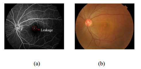
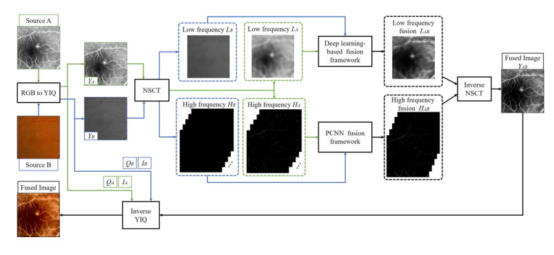
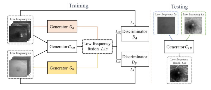
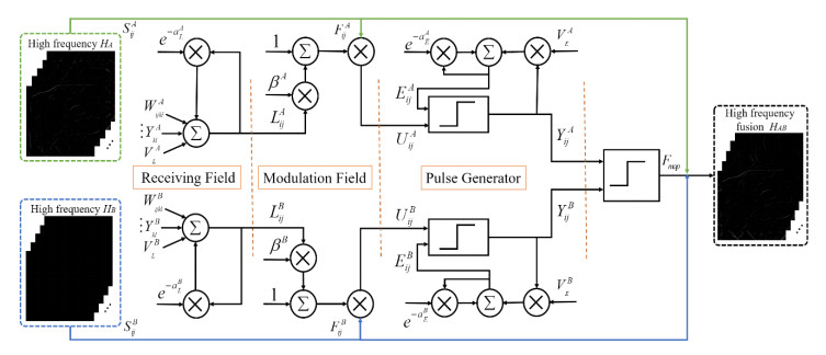
The angiography and color fundus images are of great assistance for the localization of central serous chorioretinopathy (CSCR) lesions. However, it brings much inconvenience to ophthalmologists because of these two modalities working independently in guiding laser surgery. Hence, a novel fundus image fusion method in non-subsampled contourlet transform (NSCT) domain, aiming to integrate the multi-modal CSCR information, is proposed. Specifically, the source images are initially decomposed into high-frequency and low-frequency components based on NSCT. Then, an improved deep learning-based method is employed for the fusion of low-frequency components, which helps to alleviate the tedious process of manually designing fusion rules and enhance the smoothness of the fused images. The fusion of high-frequency components based on pulse-coupled neural network (PCNN) is closely followed to facilitate the integration of detailed information. Finally, the fused images can be obtained by applying an inverse transform on the above fusion components. Qualitative and quantitative experiments demonstrate the proposed scheme is superior to the baseline methods of multi-scale transform (MST) in most cases, which not only implies its potential in multi-modal fundus image fusion, but also expands the research direction of MST-based fusion methods.
- central serous chorioretinopathy,
- image fusion,
- non-subsampled contourlet transform,
- generative adversarial network,
- pulse-coupled neural network
Citation: Jianguo Xu, Cheng Wan, Weihua Yang, Bo Zheng, Zhipeng Yan, Jianxin Shen. A novel multi-modal fundus image fusion method for guiding the laser surgery of central serous chorioretinopathy[J]. Mathematical Biosciences and Engineering, 2021, 18(4): 4797-4816. doi: 10.3934/mbe.2021244

Related Papers:

Abstract

The angiography and color fundus images are of great assistance for the localization of central serous chorioretinopathy (CSCR) lesions. However, it brings much inconvenience to ophthalmologists because of these two modalities working independently in guiding laser surgery. Hence, a novel fundus image fusion method in non-subsampled contourlet transform (NSCT) domain, aiming to integrate the multi-modal CSCR information, is proposed. Specifically, the source images are initially decomposed into high-frequency and low-frequency components based on NSCT. Then, an improved deep learning-based method is employed for the fusion of low-frequency components, which helps to alleviate the tedious process of manually designing fusion rules and enhance the smoothness of the fused images. The fusion of high-frequency components based on pulse-coupled neural network (PCNN) is closely followed to facilitate the integration of detailed information. Finally, the fused images can be obtained by applying an inverse transform on the above fusion components. Qualitative and quantitative experiments demonstrate the proposed scheme is superior to the baseline methods of multi-scale transform (MST) in most cases, which not only implies its potential in multi-modal fundus image fusion, but also expands the research direction of MST-based fusion methods.

References

[1]	A. Daruich, A. Matet, A. Dirani, E. Bousquet, M. Zhao, N. Farman, et al., Central serous chorioretinopathy: Recent findings and new physiopathology hypothesis, Prog. Retinal Eye Res., 48 (2015), 82-118. doi: 10.1016/j.preteyeres.2015.05.003
[2]	J. Yu, C. Jiang, G. Xu, Study of subretinal exudation and consequent changes in acute central serous chorioretinopathy by optical coherence tomography, Am. J. Ophthalmol., 158 (2014), 752-756. doi: 10.1016/j.ajo.2014.06.015
[3]	P. Balasubramaniam, V. P. Ananthi, Image fusion using intuitionistic fuzzy sets, Inf. Fusion, 20 (2014), 21-30. doi: 10.1016/j.inffus.2013.10.011
[4]	H. Yin, Tensor sparse representation for 3-D medical image fusion using weighted average rule, IEEE Trans. Biomed. Eng., 65 (2018), 2622-2633. doi: 10.1109/TBME.2018.2811243
[5]	J. Li, M. Song, Y. Peng, Infrared and visible image fusion based on robust principal component analysis and compressed sensing, Infrared Phys. Technol., 89 (2018), 129-139. doi: 10.1016/j.infrared.2018.01.003
[6]	Y. Leung, J. Liu, J. Zhang, An improved adaptive intensity-hue-saturation method for the fusion of remote sensing images, IEEE Geosci. Remote Sens. Lett., 11 (2014), 985-989. doi: 10.1109/LGRS.2013.2284282
[7]	Y. Yang, S. Tong, S. Huang, P. Lin, Multi-focus image fusion based on NSCT and focused area detection, IEEE Sens. J., 15 (2015), 2824-2838.
[8]	B. Yang, S. Li, Multi-focus image fusion and restoration with sparse representation, IEEE Trans. Instrum. Meas., 59 (2010), 884-892. doi: 10.1109/TIM.2009.2026612
[9]	H. Li, X. Wu, Multi-focus image fusion using dictionary learning and low-rank representation, in International Conference on Image and Graphics, Springer, 10666 (2017), 675-686.
[10]	A. B. Hamza, Y. He, H. Krim, A. Willsky, A multiscale approach to pixel-level image fusion, Integr. Comput.-Aided Eng., 12 (2005), 135-146. doi: 10.3233/ICA-2005-12201
[11]	L. Wang, B. Li, L. Tian, Multi-modal medical image fusion using the inter-scale and intra-scale dependencies between image shift-invariant shearlet coefficients, Inf. Fusion, 19 (2014), 20-28. doi: 10.1016/j.inffus.2012.03.002
[12]	M. N. Do, M. Vetterli, Contourlets: a directional multiresolution image representation, in Proceedings. International Conference on Image Processing, Rochester, NY, USA, 2002.
[13]	Z. Zhu, M. Zheng, G. Qi, D. Wang, Y. Xiang, A phase congruency and local Laplacian energy based multi-modality medical image fusion method in NSCT domain, IEEE Access, 7 (2019), 20811-20824. doi: 10.1109/ACCESS.2019.2898111
[14]	G. Easley, D. Labate, W.Q. Lim, Sparse directional image representations using the discrete shearlet transform, Appl. Comput. Harmonic Anal., 25 (2008), 25-46. doi: 10.1016/j.acha.2007.09.003
[15]	Y. Yang, Y. Que, S. Huang, P. Lin, Multimodal sensor medical image fusion based on type-2 fuzzy logic in NSCT domain, IEEE Sens. J., 16 (2016), 3735-3745. doi: 10.1109/JSEN.2016.2533864
[16]	J. Xia, Y. Chen, A. Chen, Y. Chen, Medical image fusion based on sparse representation and PCNN in NSCT domain, Comput. Math. Methods Med., 2018 (2018), 1-12.
[17]	P. Ganasala, V. Kumar, CT and MR image fusion scheme in non-subsampled contourlet transform domain, J. Digit. Imag., 27 (2014), 407-418. doi: 10.1007/s10278-013-9664-x
[18]	S. Das, M. K. Kundu, A neuro-fuzzy approach for medical image fusion, IEEE Trans. Biomed. Eng., 60 (2013), 3347-3353. doi: 10.1109/TBME.2013.2282461
[19]	A. L. D. Cunha, J. Zhou, M. N. Do, The non-subsampled contourlet transform: Theory, design, and applications, IEEE Trans. Image Process., 15 (2006), 3089-3101. doi: 10.1109/TIP.2006.877507
[20]	R. Hou, D. Zhou, R. Nie, D. Liu, L. Xiong, Y. Guo, et al., VIF-Net: an unsupervised framework for infrared and visible image fusion, IEEE Trans. Comput. Imaging, 6 (2020), 640-651. doi: 10.1109/TCI.2020.2965304
[21]	H. Li, X. Wu, J. Kittler, Infrared and visible image fusion using a deep learning framework, in 2018 24th international conference on pattern recognition (ICPR), Beijing, China, (2018), 2705-2710.
[22]	J. Ma, H. Xu, J. Jiang, X. Mei, X. Zhang, DDcGAN: A dual-discriminator conditional generative adversarial network for multi-resolution image fusion, IEEE Trans. Image Process., 29 (2020), 4980-4995. doi: 10.1109/TIP.2020.2977573
[23]	W. Kong, Y. Lei, X. Ni, Fusion technique for grey-scale visible light and infrared images based on non-subsampled contourlet transform and intensity-hue-saturation transform, IET Signal Process., 5 (2011), 75-80. doi: 10.1049/iet-spr.2009.0263
[24]	I. J. Goodfellow, J. Pouget-Abadie, M. Mirza, B. Xu, D. Warde-Farley, S. Ozair, et al., Generative adversarial networks, Adv. Neural Inf. Process. Syst., 3 (2014), 2672-2680.
[25]	S. Yu, S. Zhang, B. Wang, H. Dun, L. Xu, X. Huang, et al., Generative adversarial network based data augmentation to improve cervical cell classification model, Math. Biosci. Eng., 18 (2021), 1740-1752. doi: 10.3934/mbe.2021090
[26]	J. Ma, W. Yu, P. Liang, C. Li, J. Jiang, FusionGAN: A generative adversarial network for infrared and visible image fusion, Inf. Fusion, 48 (2019), 11-26. doi: 10.1016/j.inffus.2018.09.004
[27]	R. P. Broussard, S. K. Rogers, M. E. Oxley, G. L. Tarr, Physiologically motivated image fusion for object detection using a pulse coupled neural network, IEEE Trans. Neural Networks, 10 (1999), 554-563. doi: 10.1109/72.761712
[28]	W. Tan, P. Xiang, J. Zhang, H. Zhou, H. Qin, Remote sensing image fusion via boundary measured dual-channel pcnn in multi-scale morphological gradient domain, IEEE Access, 8 (2020), 42540-42549. doi: 10.1109/ACCESS.2020.2977299
[29]	W. Tan, W. Thitøn, P. Xiang, H. Zhou, Multi-modal brain image fusion based on multi-level edge-preserving filtering, Biomed. Signal Process. Control, 64 (2021), 102280. doi: 10.1016/j.bspc.2020.102280
[30]	D. Paquin, D. Levy, E. Schreibmann, L. Xing, Multiscale image registration, Math. Biosci. Eng., 3 (2006), 389-418. doi: 10.3934/mbe.2006.3.389
[31]	J. Wang, J. Chen, H. Xu, S. Zhang, X. Mei, J. Huang, et al., Gaussian field estimator with manifold regularization for retinal image registration, Signal Process., 157 (2019), 225-235. doi: 10.1016/j.sigpro.2018.12.004
[32]	K. Li, L. Yu, S. Wang, P. A. Heng, Unsupervised retina image synthesis via disentangled representation learning, in International Workshop on Simulation and Synthesis in Medical Imaging, Springer, Cham, 11827 (2019), 32-41.
[33]	E. M. Izhikevich, Class 1 neural excitability, conventional synapses, weakly connected networks, and mathematical foundations of pulse-coupled models, IEEE Trans. Neural Networks, 10 (1999), 499-507. doi: 10.1109/72.761707
[34]	S. Yang, M. Wang, Y. Lu, W. Qi, L. Jiao, Fusion of multi-parametric SAR images based on SW-non-subsampled contourlet and PCNN, Signal Process., 89 (2009), 2596-2608. doi: 10.1016/j.sigpro.2009.04.027
[35]	J. V. Aardt, Assessment of image fusion procedures using entropy, image quality, and multispectral classification, J. Appl. Remote Sens., 2 (2008), 023522. doi: 10.1117/1.2945910
[36]	G. Qu, D. Zhang, P. Yan, Information measure for performance of image fusion, Electron. Lett., 38 (2002), 313-315. doi: 10.1049/el:20020212
[37]	C. S. Xydeas, V. S. Petrovic, Objective image fusion performance measure, Electron. Lett., 36 (2000), 308-309. doi: 10.1049/el:20000267
[38]	B. K. S. Kumar, Multifocus and multispectral image fusion based on pixel significance using discrete cosine harmonic wavelet transform, Signal, Image Video Process., 7 (2013), 1125-1143. doi: 10.1007/s11760-012-0361-x
[39]	Z. Wang, A. C. Bovik, H. R. Sheikh, E. P. Simoncelli, Image quality assessment: From error visibility to structural similarity, IEEE Trans. Image Process., 13 (2004), 600-612. doi: 10.1109/TIP.2003.819861
[40]	H. Li, X. Wu, T. Durrani, Multi-focus noisy image fusion using low-rank representation, preprint, arXiv: 1804.09325.

Reader Comments

Your name:*

Email:*
© 2021 the Author(s), licensee AIMS Press. This is an open access article distributed under the terms of the Creative Commons Attribution License (http://creativecommons.org/licenses/by/4.0)