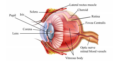
Content-based image analysis and computer vision techniques are used in various health-care systems to detect the diseases. The abnormalities in a human eye are detected through fundus images captured through a fundus camera. Among eye diseases, glaucoma is considered as the second leading case that can result in neurodegeneration illness. The inappropriate intraocular pressure within the human eye is reported as the main cause of this disease. There are no symptoms of glaucoma at earlier stages and if the disease remains unrectified then it can lead to complete blindness. The early diagnosis of glaucoma can prevent permanent loss of vision. Manual examination of human eye is a possible solution however it is dependant on human efforts. The automatic detection of glaucoma by using a combination of image processing, artificial intelligence and computer vision can help to prevent and detect this disease. In this review article, we aim to present a comprehensive review about the various types of glaucoma, causes of glaucoma, the details about the possible treatment, details about the publicly available image benchmarks, performance metrics, and various approaches based on digital image processing, computer vision, and deep learning. The review article presents a detailed study of various published research models that aim to detect glaucoma from low-level feature extraction to recent trends based on deep learning. The pros and cons of each approach are discussed in detail and tabular representations are used to summarize the results of each category. We report our findings and provide possible future research directions to detect glaucoma in conclusion.
Citation: Amsa Shabbir, Aqsa Rasheed, Huma Shehraz, Aliya Saleem, Bushra Zafar, Muhammad Sajid, Nouman Ali, Saadat Hanif Dar, Tehmina Shehryar. Detection of glaucoma using retinal fundus images: A comprehensive review[J]. Mathematical Biosciences and Engineering, 2021, 18(3): 2033-2076. doi: 10.3934/mbe.2021106
Content-based image analysis and computer vision techniques are used in various health-care systems to detect the diseases. The abnormalities in a human eye are detected through fundus images captured through a fundus camera. Among eye diseases, glaucoma is considered as the second leading case that can result in neurodegeneration illness. The inappropriate intraocular pressure within the human eye is reported as the main cause of this disease. There are no symptoms of glaucoma at earlier stages and if the disease remains unrectified then it can lead to complete blindness. The early diagnosis of glaucoma can prevent permanent loss of vision. Manual examination of human eye is a possible solution however it is dependant on human efforts. The automatic detection of glaucoma by using a combination of image processing, artificial intelligence and computer vision can help to prevent and detect this disease. In this review article, we aim to present a comprehensive review about the various types of glaucoma, causes of glaucoma, the details about the possible treatment, details about the publicly available image benchmarks, performance metrics, and various approaches based on digital image processing, computer vision, and deep learning. The review article presents a detailed study of various published research models that aim to detect glaucoma from low-level feature extraction to recent trends based on deep learning. The pros and cons of each approach are discussed in detail and tabular representations are used to summarize the results of each category. We report our findings and provide possible future research directions to detect glaucoma in conclusion.

| [1] | A. Latif, A. Rasheed, U. Sajid, J. Ahmed, N. Ali, N. I. Ratyal, et al., Content-based image retrieval and feature extraction: a comprehensive review, Math. Probl. Eng., 2019. |
| [2] |
B. Gupta, M. Tiwari, S. S. Lamba, Visibility improvement and mass segmentation of mammogram images using quantile separated histogram equalisation with local contrast enhancement, CAAI Trans. Intell. Technol., 4 (2019), 73–79. doi: 10.1049/trit.2018.1006

|
| [3] |
S. Maheshwari, V. Kanhangad, R. B. Pachori, S. V. Bhandary, U. R. Acharya, Automated glaucoma diagnosis using bit-plane slicing and local binary pattern techniques, Comput. Biol. Med., 105 (2019), 72–80. doi: 10.1016/j.compbiomed.2018.11.028
|
| [4] |
S. Masood, M. Sharif, M. Raza, M. Yasmin, M. Iqbal, M. Younus Javed, Glaucoma disease: A survey, Curr. Med. Imaging, 11 (2015), 272–283. doi: 10.2174/157340561104150727171246
|
| [5] |
U. R. Acharya, S. Bhat, J. E. Koh, S. V. Bhandary, H. Adeli, A novel algorithm to detect glaucoma risk using texton and local configuration pattern features extracted from fundus images, Comput. Biol. Med., 88 (2017), 72–83. doi: 10.1016/j.compbiomed.2017.06.022
|
| [6] |
B. J. Shingleton, L. S. Gamell, M. W. O'Donoghue, S. L. Baylus, R. King, Long-term changes in intraocular pressure after clear corneal phacoemulsification: Normal patients versus glaucoma suspect and glaucoma patients, J. Cataract. Refract. Surg., 25 (1999), 885–890. doi: 10.1016/S0886-3350(99)00107-8
|
| [7] |
K. F. Jamous, M. Kalloniatis, M. P. Hennessy, A. Agar, A. Hayen, B. Zangerl, Clinical model assisting with the collaborative care of glaucoma patients and suspects, Clin. Exp. Ophthalmol., 43 (2015), 308–319. doi: 10.1111/ceo.12466
|
| [8] | T. Khalil, M. U. Akram, S. Khalid, S. H. Dar, N. Ali, A study to identify limitations of existing automated systems to detect glaucoma at initial and curable stage, Int. J. Imaging Syst. Technol., 8 (2021). |
| [9] |
H. A. Quigley, A. T. Broman, The number of people with glaucoma worldwide in 2010 and 2020, Br. J. Ophthalmol., 90 (2006), 262–267. doi: 10.1136/bjo.2005.081224
|
| [10] |
C. Costagliola, R. Dell'Omo, M. R. Romano, M. Rinaldi, L. Zeppa, F. Parmeggiani, Pharmacotherapy of intraocular pressure: part i. parasympathomimetic, sympathomimetic and sympatholytics, Expert Opin. Pharmacother., 10 (2009), 2663–2677. doi: 10.1517/14656560903300103
|
| [11] | A. A. Salam, M. U. Akram, K. Wazir, S. M. Anwar, M. Majid, Autonomous glaucoma detection from fundus image using cup to disc ratio and hybrid features, in ISSPIT.), IEEE, 2015,370–374. |
| [12] | R. JMJ, Leading causes of blindness worldwide, Bull. Soc. Belge. Ophtalmol., 283 (2002), 19–25. |
| [13] | M. K. Dutta, A. K. Mourya, A. Singh, M. Parthasarathi, R. Burget, K. Riha, Glaucoma detection by segmenting the super pixels from fundus colour retinal images, in 2014 International Conference on Medical Imaging, m-Health and Emerging Communication Systems (MedCom.), IEEE, 2014, 86–90. |
| [14] | C. E. Willoughby, D. Ponzin, S. Ferrari, A. Lobo, K. Landau, Y. Omidi, Anatomy and physiology of the human eye: effects of mucopolysaccharidoses disease on structure and function–a review, Clin. Exp. Ophthalmol., 38 (2010), 2–11. |
| [15] |
M. S. Haleem, L. Han, J. Van Hemert, B. Li, Automatic extraction of retinal features from colour retinal images for glaucoma diagnosis: a review, Comput. Med. Imaging Graph., 37 (2013), 581–596. doi: 10.1016/j.compmedimag.2013.09.005
|
| [16] |
A. Sarhan, J. Rokne, R. Alhajj, Glaucoma detection using image processing techniques: A literature review, Comput. Med. Imaging Graph., 78 (2019), 101657. doi: 10.1016/j.compmedimag.2019.101657
|
| [17] |
H. A. Quigley, Neuronal death in glaucoma, Prog. Retin. Eye Res., 18 (1999), 39–57. doi: 10.1016/S1350-9462(98)00014-7
|
| [18] |
N. Salamat, M. M. S. Missen, A. Rashid, Diabetic retinopathy techniques in retinal images: A review, Artif. Intell. Med., 97 (2019), 168–188. doi: 10.1016/j.artmed.2018.10.009
|
| [19] | F. Bokhari, T. Syedia, M. Sharif, M. Yasmin, S. L. Fernandes, Fundus image segmentation and feature extraction for the detection of glaucoma: A new approach, Curr. Med. Imaging Rev., 14 (2018), 77–87. |
| [20] | A. Agarwal, S. Gulia, S. Chaudhary, M. K. Dutta, R. Burget, K. Riha, Automatic glaucoma detection using adaptive threshold based technique in fundus image, in (TSP.), IEEE, 2015,416–420. |
| [21] | L. Xiong, H. Li, Y. Zheng, Automatic detection of glaucoma in retinal images, in 2014 9th IEEE Conference on Industrial Electronics and Applications, IEEE, 2014, 1016–1019. |
| [22] |
A. Diaz-Pinto, S. Morales, V. Naranjo, T. Köhler, J. M. Mossi, A. Navea, Cnns for automatic glaucoma assessment using fundus images: An extensive validation, Biomed. Eng. Online, 18 (2019), 29. doi: 10.1186/s12938-019-0649-y
|
| [23] | T. Kersey, C. I. Clement, P. Bloom, M. F. Cordeiro, New trends in glaucoma risk, diagnosis & management, Indian J. Med. Res., 137 (2013), 659. |
| [24] |
A. L. Coleman, S. Miglior, Risk factors for glaucoma onset and progression, Surv. Ophthalmol., 53 (2008), S3–S10. doi: 10.1016/j.survophthal.2008.08.006
|
| [25] |
T. Saba, S. T. F. Bokhari, M. Sharif, M. Yasmin, M. Raza, Fundus image classification methods for the detection of glaucoma: A review, Microsc. Res. Tech., 81 (2018), 1105–1121. doi: 10.1002/jemt.23094
|
| [26] |
T. Aung, L. Ocaka, N. D. Ebenezer, A. G. Morris, M. Krawczak, D. L. Thiselton, et al., A major marker for normal tension glaucoma: association with polymorphisms in the opa1 gene, Hum. Genet., 110 (2002), 52–56. doi: 10.1007/s00439-001-0645-7
|
| [27] | M. A. Khaimi, Canaloplasty: A minimally invasive and maximally effective glaucoma treatment, J. Ophthalmol., 2015. |
| [28] |
M. Bechmann, M. J. Thiel, B. Roesen, S. Ullrich, M. W. Ulbig, K. Ludwig, Central corneal thickness determined with optical coherence tomography in various types of glaucoma, Br. J. Ophthalmol., 84 (2000), 1233–1237. doi: 10.1136/bjo.84.11.1233
|
| [29] |
D. Ahram, W. Alward, M. Kuehn, The genetic mechanisms of primary angle closure glaucoma, Eye., 29 (2015), 1251–1259. doi: 10.1038/eye.2015.124
|
| [30] |
R. Törnquist, Chamber depth in primary acute glaucoma, Br. J. Ophthalmol., 40 (1956), 421. doi: 10.1136/bjo.40.7.421
|
| [31] |
H. S. Sugar, F. A. Barbour, Pigmentary glaucoma*: A rare clinical entity, Am. J. Ophthalmol., 32 (1949), 90–92. doi: 10.1016/0002-9394(49)91112-5
|
| [32] |
H. S. Sugar, Pigmentary glaucoma: A 25-year review, Am. J. Ophthalmol., 62 (1966), 499–507. doi: 10.1016/0002-9394(66)91330-4
|
| [33] |
R. Ritch, U. Schlötzer-Schrehardt, A. G. Konstas, Why is glaucoma associated with exfoliation syndrome?, Prog. Retin. Eye Res., 22 (2003), 253–275. doi: 10.1016/S1350-9462(02)00014-9
|
| [34] |
J. L.-O. De, C. A. Girkin, Ocular trauma-related glaucoma., Ophthalmol. Clin. North. Am., 15 (2002), 215–223. doi: 10.1016/S0896-1549(02)00011-1
|
| [35] |
E. Milder, K. Davis, Ocular trauma and glaucoma, Int. Ophthalmol. Clin., 48 (2008), 47–64. doi: 10.1097/IIO.0b013e318187fcb8
|
| [36] |
T. G. Papadaki, I. P. Zacharopoulos, L. R. Pasquale, W. B. Christen, P. A. Netland, C. S. Foster, Long-term results of ahmed glaucoma valve implantation for uveitic glaucoma, Am. J. Ophthalmol., 144 (2007), 62–69. doi: 10.1016/j.ajo.2007.03.013
|
| [37] |
H. C. Laganowski, M. G. K. Muir, R. A. Hitchings, Glaucoma and the iridocorneal endothelial syndrome, Arch. Ophthalmol., 110 (1992), 346–350. doi: 10.1001/archopht.1992.01080150044025
|
| [38] |
C. L. Ho, D. S. Walton, Primary congenital glaucoma: 2004 update, J. Pediatr. Ophthalmol. Strabismus., 41 (2004), 271–288. doi: 10.3928/01913913-20040901-11
|
| [39] |
M. Erdurmuş, R. Yağcı, Ö. Atış, R. Karadağ, A. Akbaş, İ. F. Hepşen, Antioxidant status and oxidative stress in primary open angle glaucoma and pseudoexfoliative glaucoma, Curr. Eye Res., 36 (2011), 713–718. doi: 10.3109/02713683.2011.584370
|
| [40] |
S. S. Hayreh, Neovascular glaucoma, Prog. Retin. Eye Res., 26 (2007), 470–485. doi: 10.1016/j.preteyeres.2007.06.001
|
| [41] |
D. A. Lee, E. J. Higginbotham, Glaucoma and its treatment: a review, Am. J. Health. Syst. Pharm., 62 (2005), 691–699. doi: 10.1093/ajhp/62.7.691
|
| [42] | X. Wang, R. Khan, A. Coleman, Device-modified trabeculectomy for glaucoma, Cochrane. Database Syst. Rev.. |
| [43] |
K. R. Sung, J. S. Kim, G. Wollstein, L. Folio, M. S. Kook, J. S. Schuman, Imaging of the retinal nerve fibre layer with spectral domain optical coherence tomography for glaucoma diagnosis, Br. J. Ophthalmol., 95 (2011), 909–914. doi: 10.1136/bjo.2010.186924
|
| [44] |
M. E. Karlen, E. Sanchez, C. C. Schnyder, M. Sickenberg, A. Mermoud, Deep sclerectomy with collagen implant: medium term results, Br. J. Ophthalmol., 83 (1999), 6–11. doi: 10.1136/bjo.83.1.6
|
| [45] | J. Carrillo, L. Bautista, J. Villamizar, J. Rueda, M. Sanchez, D. Rueda, Glaucoma detection using fundus images of the eye, 2019 XXII Symposium on Image, Signal Processing and Artificial Vision (STSIVA), IEEE, 2019, 1–4. |
| [46] | N. Sengar, M. K. Dutta, R. Burget, M. Ranjoha, Automated detection of suspected glaucoma in digital fundus images, 2017 40th International Conference on Telecommunications and Signal Processing (TSP), IEEE, 2017,749–752. |
| [47] | A. Poshtyar, J. Shanbehzadeh, H. Ahmadieh, Automatic measurement of cup to disc ratio for diagnosis of glaucoma on retinal fundus images, in 2013 6th International Conference on Biomedical Engineering and Informatics, IEEE, 2013, 24–27. |
| [48] | F. Khan, S. A. Khan, U. U. Yasin, I. ul Haq, U. Qamar, Detection of glaucoma using retinal fundus images, in The 6th 2013 Biomedical Engineering International Conference, IEEE, 2013, 1–5. |
| [49] |
H. Yamada, T. Akagi, H. Nakanishi, H. O. Ikeda, Y. Kimura, K. Suda, et al., Microstructure of peripapillary atrophy and subsequent visual field progression in treated primary open-angle glaucoma, Ophthalmology, 123 (2016), 542–551. doi: 10.1016/j.ophtha.2015.10.061
|
| [50] |
J. B. Jonas, Clinical implications of peripapillary atrophy in glaucoma, Curr. Opin. Ophthalmol., 16 (2005), 84–88. doi: 10.1097/01.icu.0000156135.20570.30
|
| [51] |
K. H. Park, G. Tomita, S. Y. Liou, Y. Kitazawa, Correlation between peripapillary atrophy and optic nerve damage in normal-tension glaucoma, Ophthalmol., 103 (1996), 1899–1906. doi: 10.1016/S0161-6420(96)30409-0
|
| [52] |
F. A. Medeiros, L. M. Zangwill, C. Bowd, R. M. Vessani, R. Susanna Jr, R. N. Weinreb, Evaluation of retinal nerve fiber layer, optic nerve head, and macular thickness measurements for glaucoma detection using optical coherence tomography, Am. J. Ophthalmol., 139 (2005), 44–55. doi: 10.1016/j.ajo.2004.08.069
|
| [53] |
G. Wollstein, J. S. Schuman, L. L. Price, A. Aydin, P. C. Stark, E. Hertzmark, et al., Optical coherence tomography longitudinal evaluation of retinal nerve fiber layer thickness in glaucoma, Arch. Ophthalmol., 123 (2005), 464–470. doi: 10.1001/archopht.123.4.464
|
| [54] |
M. Armaly, The optic cup in the normal eye: I. cup width, depth, vessel displacement, ocular tension and outflow facility, Am. J. Ophthalmol., 68 (1969), 401–407. doi: 10.1016/0002-9394(69)90702-8
|
| [55] | M. Galdos, A. Bayon, F. D. Rodriguez, C. Mico, S. C. Sharma, E. Vecino, Morphology of retinal vessels in the optic disk in a göttingen minipig experimental glaucoma model, Vet. Ophthalmol., 15 (2012), 36–46. |
| [56] | W. Zhou, Y. Yi, Y. Gao, J. Dai, Optic disc and cup segmentation in retinal images for glaucoma diagnosis by locally statistical active contour model with structure prior, Comput. Math. Methods. Med., 2019. |
| [57] |
P. Sharma, P. A. Sample, L. M. Zangwill, J. S. Schuman, Diagnostic tools for glaucoma detection and management, Surv. Ophthalmol., 53 (2008), S17–S32. doi: 10.1016/j.survophthal.2008.08.003
|
| [58] | M. J. Greaney, D. C. Hoffman, D. F. Garway-Heath, M. Nakla, A. L. Coleman, J. Caprioli, Comparison of optic nerve imaging methods to distinguish normal eyes from those with glaucoma, Invest. Ophthalmol. Vis. Sci., 43 (2002), 140–145. |
| [59] |
R. Bock, J. Meier, L. G. Nyúl, J. Hornegger, G. Michelson, Glaucoma risk index: automated glaucoma detection from color fundus images, Med. Image. Anal., 14 (2010), 471–481. doi: 10.1016/j.media.2009.12.006
|
| [60] |
K. Chan, T.-W. Lee, P. A. Sample, M. H. Goldbaum, R. N. Weinreb, T. J. Sejnowski, Comparison of machine learning and traditional classifiers in glaucoma diagnosis, IEEE Trans. Biomed. Eng., 49 (2002), 963–974. doi: 10.1109/TBME.2002.802012
|
| [61] | N. Varachiu, C. Karanicolas, M. Ulieru, Computational intelligence for medical knowledge acquisition with application to glaucoma, in Proceedings First IEEE International Conference on Cognitive Informatics, IEEE, 2002,233–238. |
| [62] | J. Yu, S. S. R. Abidi, P. H. Artes, A. McIntyre, M. Heywood, Automated optic nerve analysis for diagnostic support inglaucoma, in CBMS'05., IEEE, 2005, 97–102. |
| [63] | R. Bock, J. Meier, G. Michelson, L. G. Nyúl and J. Hornegger, Classifying glaucoma with image-based features from fundus photographs, in Joint Pattern Recognition Symposium., Springer, 2007,355–364. |
| [64] | Y. Hatanaka, A. Noudo, C. Muramatsu, A. Sawada, T. Hara, T. Yamamoto, et al., Vertical cup-to-disc ratio measurement for diagnosis of glaucoma on fundus images, in Medical Imaging 2010: Computer-Aided Diagnosis, vol. 7624, International Society for Optics and Photonics, 2010, 76243C. |
| [65] | S. S. Abirami, S. G. Shoba, Glaucoma images classification using fuzzy min-max neural network based on data-core, IJISME., 1 (2013), 9–15. |
| [66] |
J. Liu, Z. Zhang, D. W. K. Wong, Y. Xu, F. Yin, J. Cheng, et al., Automatic glaucoma diagnosis through medical imaging informatics, Journal of the American Medical Informatics Association, 20 (2013), 1021–1027. doi: 10.1136/amiajnl-2012-001336
|
| [67] | A. Almazroa, R. Burman, K. Raahemifar, V. Lakshminarayanan, Optic disc and optic cup segmentation methodologies for glaucoma image detection: A survey, J. Ophthalmol., 2015. |
| [68] | A. Dey, S. K. Bandyopadhyay, Automated glaucoma detection using support vector machine classification method, J. Adv. Med. Med. Res., 1–12. |
| [69] |
F. R. Silva, V. G. Vidotti, F. Cremasco, M. Dias, E. S. Gomi, V. P. Costa, Sensitivity and specificity of machine learning classifiers for glaucoma diagnosis using spectral domain oct and standard automated perimetry, Arq. Bras. Oftalmol., 76 (2013), 170–174. doi: 10.1590/S0004-27492013000300008
|
| [70] |
M. U. Akram, A. Tariq, S. Khalid, M. Y. Javed, S. Abbas, U. U. Yasin, Glaucoma detection using novel optic disc localization, hybrid feature set and classification techniques, Australas. Phys. Eng. Sci. Med., 38 (2015), 643–655. doi: 10.1007/s13246-015-0377-y
|
| [71] | A. T. A. Al-Sammarraie, R. R. Jassem, T. K. Ibrahim, Mixed convection heat transfer in inclined tubes with constant heat flux, Eur. J. Sci. Res., 97 (2013), 144–158. |
| [72] |
M. R. K. Mookiah, U. R. Acharya, C. M. Lim, A. Petznick, J. S. Suri, Data mining technique for automated diagnosis of glaucoma using higher order spectra and wavelet energy features, Knowl. Based. Syst., 33 (2012), 73–82. doi: 10.1016/j.knosys.2012.02.010
|
| [73] | C. Raja, N. Gangatharan, Glaucoma detection in fundal retinal images using trispectrum and complex wavelet-based features, Eur. J. Sci. Res., 97 (2013), 159–171. |
| [74] | G. Lim, Y. Cheng, W. Hsu, M. L. Lee, Integrated optic disc and cup segmentation with deep learning, in ICTAI., IEEE, 2015,162–169. |
| [75] | K.-K. Maninis, J. Pont-Tuset, P. Arbeláez, L. Van Gool, Deep retinal image understanding, in International conference on medical image computing and computer-assisted intervention, Springer, 2016,140–148. |
| [76] |
B. Al-Bander, W. Al-Nuaimy, B. M. Williams, Y. Zheng, Multiscale sequential convolutional neural networks for simultaneous detection of fovea and optic disc, Biomed. Signal Process Control., 40 (2018), 91–101. doi: 10.1016/j.bspc.2017.09.008
|
| [77] |
A. Mitra, P. S. Banerjee, S. Roy, S. Roy, S. K. Setua, The region of interest localization for glaucoma analysis from retinal fundus image using deep learning, Comput. Methods Programs Biomed., 165 (2018), 25–35. doi: 10.1016/j.cmpb.2018.08.003
|
| [78] |
S. S. Kruthiventi, K. Ayush, R. V. Babu, Deepfix: A fully convolutional neural network for predicting human eye fixations, IEEE Trans. Image. Process., 26 (2017), 4446–4456. doi: 10.1109/TIP.2017.2710620
|
| [79] | M. Norouzifard, A. Nemati, A. Abdul-Rahman, H. GholamHosseini, R. Klette, A comparison of transfer learning techniques, deep convolutional neural network and multilayer neural network methods for the diagnosis of glaucomatous optic neuropathy, in International Computer Symposium, Springer, 2018,627–635. |
| [80] | X. Sun, Y. Xu, W. Zhao, T. You, J. Liu, Optic disc segmentation from retinal fundus images via deep object detection networks, in EMBC., IEEE, 2018, 5954–5957. |
| [81] | Z. Ghassabi, J. Shanbehzadeh, K. Nouri-Mahdavi, A unified optic nerve head and optic cup segmentation using unsupervised neural networks for glaucoma screening, in EMBC., IEEE, 2018, 5942–5945. |
| [82] |
J. H. Tan, S. V. Bhandary, S. Sivaprasad, Y. Hagiwara, A. Bagchi, U. Raghavendra, et al., Age-related macular degeneration detection using deep convolutional neural network, Future Gener. Comput. Syst., 87 (2018), 127–135. doi: 10.1016/j.future.2018.05.001
|
| [83] |
J. Zilly, J. M. Buhmann, D. Mahapatra, Glaucoma detection using entropy sampling and ensemble learning for automatic optic cup and disc segmentation, Comput. Med. Imaging Graph., 55 (2017), 28–41. doi: 10.1016/j.compmedimag.2016.07.012
|
| [84] |
J. Cheng, J. Liu, Y. Xu, F. Yin, D. W. K. Wong, N.-M. Tan, et al., Superpixel classification based optic disc and optic cup segmentation for glaucoma screening, IEEE Trans. Med. Imaging, 32 (2013), 1019–1032. doi: 10.1109/TMI.2013.2247770
|
| [85] | H. Ahmad, A. Yamin, A. Shakeel, S. O. Gillani, U. Ansari, Detection of glaucoma using retinal fundus images, in iCREATE., IEEE, 2014,321–324. |
| [86] | S. Kavitha, S. Karthikeyan, K. Duraiswamy, Neuroretinal rim quantification in fundus images to detect glaucoma, IJCSNS., 10 (2010), 134–140. |
| [87] | Z. Zhang, B. H. Lee, J. Liu, D. W. K. Wong, N. M. Tan, J. H. Lim, et al., Optic disc region of interest localization in fundus image for glaucoma detection in argali, in 2010 5th IEEE Conference on Industrial Electronics and Applications, IEEE, 2010, 1686–1689. |
| [88] |
D. Welfer, J. Scharcanski, C. M. Kitamura, M. M. Dal Pizzol, L. W. Ludwig, D. R. Marinho, Segmentation of the optic disk in color eye fundus images using an adaptive morphological approach, Computers Biol. Med., 40 (2010), 124–137. doi: 10.1016/j.compbiomed.2009.11.009
|
| [89] |
H. Tjandrasa, A. Wijayanti, N. Suciati, Optic nerve head segmentation using hough transform and active contours, Telkomnika, 10 (2012), 531. doi: 10.12928/telkomnika.v10i3.833
|
| [90] | M. Tavakoli, M. Nazar, A. Golestaneh, F. Kalantari, Automated optic nerve head detection based on different retinal vasculature segmentation methods and mathematical morphology, in NSS/MIC., IEEE, 2017, 1–7. |
| [91] |
P. Bibiloni, M. González-Hidalgo, S. Massanet, A real-time fuzzy morphological algorithm for retinal vessel segmentation, J. Real Time Image Process., 16 (2019), 2337–2350. doi: 10.1007/s11554-018-0748-1
|
| [92] | A. Agarwal, A. Issac, A. Singh, M. K. Dutta, Automatic imaging method for optic disc segmentation using morphological techniques and active contour fitting, in 2016 Ninth International Conference on Contemporary Computing (IC3), IEEE, 2016, 1–5. |
| [93] | S. Pal, S. Chatterjee, Mathematical morphology aided optic disk segmentation from retinal images, in 2017 3rd International Conference on Condition Assessment Techniques in Electrical Systems (CATCON), IEEE, 2017,380–385. |
| [94] | L. Wang, A. Bhalerao, Model based segmentation for retinal fundus images, in Scandinavian Conference on Image Analysis, Springer, 2003,422–429. |
| [95] | G. Deng, L. Cahill, An adaptive gaussian filter for noise reduction and edge detection, in 1993 IEEE conference record nuclear science symposium and medical imaging conference, IEEE, 1993, 1615–1619. |
| [96] |
K. A. Vermeer, F. M. Vos, H. G. Lemij, A. M. Vossepoel, A model based method for retinal blood vessel detection, Comput. Biol. Med., 34 (2004), 209–219. doi: 10.1016/S0010-4825(03)00055-6
|
| [97] | J. I. Orlando, E. Prokofyeva, M. B. Blaschko, A discriminatively trained fully connected conditional random field model for blood vessel segmentation in fundus images, IEEE Trans. Biomed. Eng., 64 (2016), 16–27. |
| [98] | R. Ingle, P. Mishra, Cup segmentation by gradient method for the assessment of glaucoma from retinal image, Int. J. Latest Trends. Eng. Technol., 4 (2013), 2540–2543. |
| [99] | G. D. Joshi, J. Sivaswamy, S. Krishnadas, Optic disk and cup segmentation from monocular color retinal images for glaucoma assessment, IEEE Trans. Biomed. Eng., 30 (2011), 1192–1205. |
| [100] | W. W. K. Damon, J. Liu, T. N. Meng, Y. Fengshou, W. T. Yin, Automatic detection of the optic cup using vessel kinking in digital retinal fundus images, in 2012 9th IEEE International Symposium on Biomedical Imaging (ISBI), IEEE, 2012, 1647–1650. |
| [101] | D. Finkelstein, Kinks, J. Math. Phys., 7 (1966), 1218–1225. |
| [102] | Y. Xu, L. Duan, S. Lin, X. Chen, D. W. K. Wong, T. Y. Wong, et al., Optic cup segmentation for glaucoma detection using low-rank superpixel representation, in International Conference on Medical Image Computing and Computer-Assisted Intervention, Springer, 2014,788–795. |
| [103] | Y. Xu, J. Liu, S. Lin, D. Xu, C. Y. Cheung, T. Aung, et al., Efficient optic cup detection from intra-image learning with retinal structure priors, in International Conference on Medical Image Computing and Computer-Assisted Intervention, Springer, 2012, 58–65. |
| [104] | M. A. Aslam, M. N. Salik, F. Chughtai, N. Ali, S. H. Dar, T. Khalil, Image classification based on mid-level feature fusion, in 2019 15th International Conference on Emerging Technologies (ICET), IEEE, 2019, 1–6. |
| [105] |
N. Ali, K. B. Bajwa, R. Sablatnig, S. A. Chatzichristofis, Z. Iqbal, M. Rashid, et al., A novel image retrieval based on visual words integration of sift and surf, PloS. one., 11 (2016), e0157428. doi: 10.1371/journal.pone.0157428
|
| [106] | C.-Y. Ho, T.-W. Pai, H.-T. Chang, H.-Y. Chen, An atomatic fundus image analysis system for clinical diagnosis of glaucoma, in 2011 International Conference on Complex, Intelligent, and Software Intensive Systems, IEEE, 2011,559–564. |
| [107] |
H.-T. Chang, C.-H. Liu, T.-W. Pai, Estimation and extraction of b-cell linear epitopes predicted by mathematical morphology approaches, J. Mol. Recognit., 21 (2008), 431–441. doi: 10.1002/jmr.910
|
| [108] | D. Wong, J. Liu, J. Lim, N. Tan, Z. Zhang, S. Lu, et al., Intelligent fusion of cup-to-disc ratio determination methods for glaucoma detection in argali, in 2009 Annual International Conference of the IEEE Engineering in Medicine and Biology Society, IEEE, 2009, 5777–5780. |
| [109] | F. Yin, J. Liu, D. W. K. Wong, N. M. Tan, C. Cheung, M. Baskaran, et al., Automated segmentation of optic disc and optic cup in fundus images for glaucoma diagnosis, in 2012 25th IEEE international symposium on computer-based medical systems (CBMS), IEEE, 2012, 1–6. |
| [110] | S. Chandrika, K. Nirmala, Analysis of cdr detection for glaucoma diagnosis, IJERA., 2 (2013), 23–27. |
| [111] | N. Annu, J. Justin, Automated classification of glaucoma images by wavelet energy features, IJERA., 5 (2013), 1716–1721. |
| [112] |
H. Fu, J. Cheng, Y. Xu, D. W. K. Wong, J. Liu, X. Cao, Joint optic disc and cup segmentation based on multi-label deep network and polar transformation, IEEE Trans. Med. Imaging., 37 (2018), 1597–1605. doi: 10.1109/TMI.2018.2791488
|
| [113] | P. K. Dhar, T. Shimamura, Blind svd-based audio watermarking using entropy and log-polar transformation, JISA., 20 (2015), 74–83. |
| [114] | D. Wong, J. Liu, J. Lim, H. Li, T. Wong, Automated detection of kinks from blood vessels for optic cup segmentation in retinal images, in Medical Imaging 2009: Computer-Aided Diagnosis, vol. 7260, International Society for Optics and Photonics, 2009, 72601J. |
| [115] | A. Murthi, M. Madheswaran, Enhancement of optic cup to disc ratio detection in glaucoma diagnosis, in 2012 International Conference on Computer Communication and Informatics, IEEE, 2012, 1–5. |
| [116] |
N. E. A. Khalid, N. M. Noor, N. M. Ariff, Fuzzy c-means (fcm) for optic cup and disc segmentation with morphological operation, Procedia. Comput. Sci., 42 (2014), 255–262. doi: 10.1016/j.procs.2014.11.060
|
| [117] | H. A. Nugroho, W. K. Oktoeberza, A. Erasari, A. Utami, C. Cahyono, Segmentation of optic disc and optic cup in colour fundus images based on morphological reconstruction, in 2017 9th International Conference on Information Technology and Electrical Engineering (ICITEE), IEEE, 2017, 1–5. |
| [118] |
L. Zhang, M. Fisher, W. Wang, Retinal vessel segmentation using multi-scale textons derived from keypoints, Comput. Med. Imaging Graph., 45 (2015), 47–56. doi: 10.1016/j.compmedimag.2015.07.006
|
| [119] | X. Li, B. Aldridge, R. Fisher, J. Rees, Estimating the ground truth from multiple individual segmentations incorporating prior pattern analysis with application to skin lesion segmentation, in 2011 IEEE International Symposium on Biomedical Imaging: From Nano to Macro, IEEE, 2011, 1438–1441. |
| [120] | M. M. Fraz, P. Remagnino, A. Hoppe, S. Velastin, B. Uyyanonvara, S. Barman, A supervised method for retinal blood vessel segmentation using line strength, multiscale gabor and morphological features, in 2011 IEEE International Conference on Signal and Image Processing Applications (ICSIPA), IEEE, 2011,410–415. |
| [121] | M. Niemeijer, J. Staal, B. van Ginneken, M. Loog, M. D. Abramoff, Comparative study of retinal vessel segmentation methods on a new publicly available database, in Medical imaging 2004: Image processing, vol. 5370, International Society for Optics and Photonics, 2004,648–656. |
| [122] | J. Y. Choi, T. K. Yoo, J. G. Seo, J. Kwak, T. T. Um, T. H. Rim, Multi-categorical deep learning neural network to classify retinal images: a pilot study employing small database, PloS one, 12. |
| [123] | L. Zhang, M. Fisher, W. Wang, Comparative performance of texton based vascular tree segmentation in retinal images, in 2014 IEEE International Conference on Image Processing (ICIP), IEEE, 2014,952–956. |
| [124] |
A. Septiarini, A. Harjoko, R. Pulungan, R. Ekantini, Automated detection of retinal nerve fiber layer by texture-based analysis for glaucoma evaluation, Healthc. Inform. Res., 24 (2018), 335–345. doi: 10.4258/hir.2018.24.4.335
|
| [125] | B. S. Kirar, D. K. Agrawal, Computer aided diagnosis of glaucoma using discrete and empirical wavelet transform from fundus images, IET Image Process., 13 (2018), 73–82. |
| [126] | K. Nirmala, N. Venkateswaran, C. V. Kumar, J. S. Christobel, Glaucoma detection using wavelet based contourlet transform, in 2017 International Conference on Intelligent Computing and Control (I2C2), IEEE, 2017, 1–5. |
| [127] |
A. A. G. Elseid, A. O. Hamza, Glaucoma detection using retinal nerve fiber layer texture features, J. Clin. Eng., 44 (2019), 180–185. doi: 10.1097/JCE.0000000000000361
|
| [128] | M. Claro, L. Santos, W. Silva, F. Araújo, N. Moura, A. Macedo, Automatic glaucoma detection based on optic disc segmentation and texture feature extraction, CLEI Electron. J., 19 (2016), 5. |
| [129] | L. Abdel-Hamid, Glaucoma detection from retinal images using statistical and textural wavelet features, J. Digit Imaging., 1–8. |
| [130] |
S. Maetschke, B. Antony, H. Ishikawa, G. Wollstein, J. Schuman, R. Garnavi, A feature agnostic approach for glaucoma detection in oct volumes, PloS. one., 14 (2019), e0219126. doi: 10.1371/journal.pone.0219915
|
| [131] |
D. C. Hood, A. S. Raza, On improving the use of oct imaging for detecting glaucomatous damage, Br. J. Ophthalmol., 98 (2014), ii1–ii9. doi: 10.1136/bjophthalmol-2014-305156
|
| [132] |
D. C. Hood, Improving our understanding, and detection, of glaucomatous damage: an approach based upon optical coherence tomography (oct), Prog.Retin. Eye Res., 57 (2017), 46–75. doi: 10.1016/j.preteyeres.2016.12.002
|
| [133] |
H. S. Basavegowda, G. Dagnew, Deep learning approach for microarray cancer data classification, CAAI Trans. Intell. Technol., 5 (2020), 22–33. doi: 10.1049/trit.2019.0028
|
| [134] | X. Chen, Y. Xu, D. W. K. Wong, T. Y. Wong, J. Liu, Glaucoma detection based on deep convolutional neural network, in 2015 37th annual international conference of the IEEE engineering in medicine and biology society (EMBC), IEEE, 2015,715–718. |
| [135] |
U. T. Nguyen, A. Bhuiyan, L. A. Park, K. Ramamohanarao, An effective retinal blood vessel segmentation method using multi-scale line detection, Pattern Recognit., 46 (2013), 703–715. doi: 10.1016/j.patcog.2012.08.009
|
| [136] |
J. H. Tan, U. R. Acharya, S. V. Bhandary, K. C. Chua, S. Sivaprasad, Segmentation of optic disc, fovea and retinal vasculature using a single convolutional neural network, J. Comput. Sci., 20 (2017), 70–79. doi: 10.1016/j.jocs.2017.02.006
|
| [137] |
Y. Chai, H. Liu, J. Xu, Glaucoma diagnosis based on both hidden features and domain knowledge through deep learning models, Knowl. Based Syst., 161 (2018), 147–156. doi: 10.1016/j.knosys.2018.07.043
|
| [138] | A. Pal, M. R. Moorthy, A. Shahina, G-eyenet: A convolutional autoencoding classifier framework for the detection of glaucoma from retinal fundus images, in 2018 25th IEEE International Conference on Image Processing (ICIP), IEEE, 2018, 2775–2779. |
| [139] |
R. Asaoka, M. Tanito, N. Shibata, K. Mitsuhashi, K. Nakahara, Y. Fujino, et al., Validation of a deep learning model to screen for glaucoma using images from different fundus cameras and data augmentation, Ophthalmol. Glaucoma., 2 (2019), 224–231. doi: 10.1016/j.ogla.2019.03.008
|
| [140] | X. Chen, Y. Xu, S. Yan, D. W. K. Wong, T. Y. Wong, J. Liu, Automatic feature learning for glaucoma detection based on deep learning, in International Conference on Medical Image Computing and Computer-Assisted Intervention, Springer, 2015,669–677. |
| [141] | A. Singh, S. Sengupta, V. Lakshminarayanan, Glaucoma diagnosis using transfer learning methods, in Applications of Machine Learning, vol. 11139, International Society for Optics and Photonics, 2019, 111390U. |
| [142] | S. Maheshwari, V. Kanhangad, R. B. Pachori, Cnn-based approach for glaucoma diagnosis using transfer learning and lbp-based data augmentation, arXiv. preprint. |
| [143] |
S. Sengupta, A. Singh, H. A. Leopold, T. Gulati, V. Lakshminarayanan, Ophthalmic diagnosis using deep learning with fundus images–a critical review, Artif. Intell. Med., 102 (2020), 101758. doi: 10.1016/j.artmed.2019.101758
|
| [144] |
U. Raghavendra, H. Fujita, S. V. Bhandary, A. Gudigar, J. H. Tan, U. R. Acharya, Deep convolution neural network for accurate diagnosis of glaucoma using digital fundus images, Inf. Sci., 441 (2018), 41–49. doi: 10.1016/j.ins.2018.01.051
|
| [145] |
R. Asaoka, H. Murata, A. Iwase, M. Araie, Detecting preperimetric glaucoma with standard automated perimetry using a deep learning classifier, Ophthalmol., 123 (2016), 1974–1980. doi: 10.1016/j.ophtha.2016.05.029
|
| [146] |
Z. Li, Y. He, S. Keel, W. Meng, R. T. Chang, M. He, Efficacy of a deep learning system for detecting glaucomatous optic neuropathy based on color fundus photographs, Ophthalmol., 125 (2018), 1199–1206. doi: 10.1016/j.ophtha.2018.01.023
|
| [147] | V. V. Raghavan, V. N. Gudivada, V. Govindaraju, C. R. Rao, Cognitive computing: Theory and applications, Elsevier., 2016. |
| [148] | J. Sivaswamy, S. Krishnadas, G. D. Joshi, M. Jain, A. U. S. Tabish, Drishti-gs: Retinal image dataset for optic nerve head (onh) segmentation, in 2014 IEEE 11th international symposium on biomedical imaging (ISBI), IEEE, 2014, 53–56. |
| [149] | A. Chakravarty, J. Sivaswamy, Glaucoma classification with a fusion of segmentation and image-based features, in 2016 IEEE 13th international symposium on biomedical imaging (ISBI), IEEE, 2016,689–692. |
| [150] |
E. Decencière, X. Zhang, G. Cazuguel, B. Lay, B. Cochener, C. Trone, et al., Feedback on a publicly distributed image database: The messidor database, Image Analys. Stereol., 33 (2014), 231–234. doi: 10.5566/ias.1155
|
| [151] |
A. Allam, A. Youssif, A. Ghalwash, Automatic segmentation of optic disc in eye fundus images: a survey, ELCVIA, 14 (2015), 1–20. doi: 10.5565/rev/elcvia.762
|
| [152] |
P. Porwal, S. Pachade, R. Kamble, M. Kokare, G. Deshmukh, V. Sahasrabuddhe, et al., Indian diabetic retinopathy image dataset (idrid): A database for diabetic retinopathy screening research, Data, 3 (2018), 25. doi: 10.3390/data3030025
|
| [153] | F. Calimeri, A. Marzullo, C. Stamile, G. Terracina, Optic disc detection using fine tuned convolutional neural networks, in 2016 12th International Conference on Signal-Image Technology & Internet-Based Systems (SITIS), IEEE, 2016, 69–75. |
| [154] |
M. N. Reza, Automatic detection of optic disc in color fundus retinal images using circle operator, Biomed. Signal. Process. Control., 45 (2018), 274–283. doi: 10.1016/j.bspc.2018.05.027
|
| [155] | Z. Zhang, F. S. Yin, J. Liu, W. K. Wong, N. M. Tan, B. H. Lee, et al., Origa-light: An online retinal fundus image database for glaucoma analysis and research, in 2010 Annual International Conference of the IEEE Engineering in Medicine and Biology, IEEE, 2010, 3065–3068. |
| [156] | Z. Zhang, J. Liu, F. Yin, B.-H. Lee, D. W. K. Wong, K. R. Sung, Achiko-k: Database of fundus images from glaucoma patients, in 2013 IEEE 8th Conference on Industrial Electronics and Applications (ICIEA), IEEE, 2013,228–231. |
| [157] | F. Yin, J. Liu, D. W. K. Wong, N. M. Tan, B. H. Lee, J. Cheng, et al., Achiko-i retinal fundus image database and its evaluation on cup-to-disc ratio measurement, in 2013 IEEE 8th Conference on Industrial Electronics and Applications (ICIEA), IEEE, 2013,224–227. |
| [158] | F. Fumero, S. Alayón, J. L. Sanchez, J. Sigut, M. Gonzalez-Hernandez, Rim-one: An open retinal image database for optic nerve evaluation, in 2011 24th international symposium on computer-based medical systems (CBMS), IEEE, 2011, 1–6. |
| [159] |
J. Lowell, A. Hunter, D. Steel, A. Basu, R. Ryder, E. Fletcher, et al., Optic nerve head segmentation, IEEE Trans. Med. Imaging., 23 (2004), 256–264. doi: 10.1109/TMI.2003.823261
|
| [160] |
C. C. Sng, L.-L. Foo, C.-Y. Cheng, J. C. Allen Jr, M. He, G. Krishnaswamy, et al., Determinants of anterior chamber depth: the singapore chinese eye study, Ophthalmol., 119 (2012), 1143–1150. doi: 10.1016/j.ophtha.2012.01.011
|
| [161] | Z. Zhang, J. Liu, C. K. Kwoh, X. Sim, W. T. Tay, Y. Tan, et al., Learning in glaucoma genetic risk assessment, in 2010 Annual International Conference of the IEEE Engineering in Medicine and Biology, IEEE, 2010, 6182–6185. |
| [162] | D. Wong, J. Liu, J. Lim, X. Jia, F. Yin, H. Li, et al., Level-set based automatic cup-to-disc ratio determination using retinal fundus images in argali, in 2008 30th Annual International Conference of the IEEE Engineering in Medicine and Biology Society, IEEE, 2008, 2266–2269. |
| [163] | T. Ge, L. Cui, B. Chang, Z. Sui, F. Wei, M. Zhou, Seri: A dataset for sub-event relation inference from an encyclopedia, in CCF International Conference on Natural Language Processing and Chinese Computing, Springer, 2018,268–277. |
| [164] | M. Haloi, Improved microaneurysm detection using deep neural networks, arXiv. preprint.. |
| [165] |
B. Antal, A. Hajdu, An ensemble-based system for automatic screening of diabetic retinopathy, Knowl. Based Syst., 60 (2014), 20–27. doi: 10.1016/j.knosys.2013.12.023
|
| [166] |
J. Nayak, R. Acharya, P. S. Bhat, N. Shetty, T.-C. Lim, Automated diagnosis of glaucoma using digital fundus images, J. Med. Syst., 33 (2009), 337. doi: 10.1007/s10916-008-9195-z
|
| [167] |
J. V. Soares, J. J. Leandro, R. M. Cesar, H. F. Jelinek, M. J. Cree, Retinal vessel segmentation using the 2-d gabor wavelet and supervised classification, IEEE Trans. Med. Imaging., 25 (2006), 1214–1222. doi: 10.1109/TMI.2006.879967
|
| [168] |
S. Kankanahalli, P. M. Burlina, Y. Wolfson, D. E. Freund, N. M. Bressler, Automated classification of severity of age-related macular degeneration from fundus photographs, Invest. Ophthalmol. Vis. Sci., 54 (2013), 1789–1796. doi: 10.1167/iovs.12-10928
|
| [169] | K. Prasad, P. Sajith, M. Neema, L. Madhu, P. Priya, Multiple eye disease detection using deep neural network, in TENCON 2019-2019 IEEE Region 10 Conference (TENCON), IEEE, 2019, 2148–2153. |
Figures(12) / Tables(15)

Amsa Shabbir, Aqsa Rasheed, Huma Shehraz, Aliya Saleem, Bushra Zafar, Muhammad Sajid, Nouman Ali, Saadat Hanif Dar, Tehmina Shehryar. Detection of glaucoma using retinal fundus images: A comprehensive review[J]. Mathematical Biosciences and Engineering, 2021, 18(3): 2033-2076. doi: 10.3934/mbe.2021106


 DownLoad: