Federated and ensemble learning framework with optimized feature selection for heart disease detection

Olfa Hrizi; Karim Gasmi; Abdulrahman Alyami; Adel Alkhalil; Ibrahim Alrashdi; Ali Alqazzaz; Lassaad Ben Ammar; Manel Mrabet; Alameen E.M. Abdalrahman; Samia Yahyaoui; Olfa Hrizi; Karim Gasmi; Abdulrahman Alyami; Adel Alkhalil; Ibrahim Alrashdi; Ali Alqazzaz; Lassaad Ben Ammar; Manel Mrabet; Alameen E.M. Abdalrahman; Samia Yahyaoui

doi:10.3934/math.2025334

AIMS Mathematics

2025, Volume 10, Issue 3: 7290-7318. doi: 10.3934/math.2025334

Previous Article Next Article

Research article Special Issues

Federated and ensemble learning framework with optimized feature selection for heart disease detection

1.
Department of Computer Science, College of Computer and Information Sciences, Jouf University, Sakaka 72388, Saudi Arabia
2.
Department of Information Systems, College of Computer and Information Sciences, Jouf University, Sakaka, Saudi Arabia
3.
Department of Software Engineering, College of Computer Science and Engineering, University of Hail, Hail, 81481 Saudi Arabia
4.
College of Computing and Information Technology, University of Bisha, Bisha 61922, Saudi Arabia
5.
Prince Sattam bin Abdulaziz University, Al-Kharj, Saudi Arabia
6.
Department of Physics, College of Science, Jouf University, Sakaka, Aljouf 72341, Saudi Arabia

Received: 08 February 2025 Revised: 17 March 2025 Accepted: 24 March 2025 Published: 28 March 2025
MSC : 62H30, 68T05, 92C50, 68U35, 90C59

Predictive models for early identification of heart disease must be precise and efficient because it is a major worldwide health concern. To improve classification performance while protecting data privacy, this study investigated a combined method that uses ensemble learning, feature selection, and federated learning (FL). The ensemble-based approaches proved the most predictive after testing several different machine learning (ML) models, including random forests, the light gradient boosting machine, support vector machines, k-nearest neighbors, convolutional neural networks, and long short-term memory. We used particle swarm optimization (PSO) for feature selection, which optimized the most relevant features in conjunction with voting and stacking approaches to further increase the model's performance. In addition, federated learning was implemented to allow decentralized training while preserving sensitive medical data. The results highlight the effectiveness of combining these techniques in the detection of heart disease, providing a scalable and privacy-preserving solution for real-world healthcare applications. Two benchmark datasets were used to validate the proposed approach, ensuring the reliability and generalizability of the findings. Furthermore, we used four performance metrics, namely accuracy, precision, recall, and F1score, to evaluate the selected models. Finally, federated learning was included to handle privacy issues and guarantee safe access to private medical data. This distributed method allows model training without centralizing patient data, so it is compatible with strict data privacy rules. With up to 95% precision, our method shows a notable increase in prediction accuracy according to the testing results. This work offers a strong, scalable, and safe solution for the early identification of cardiovascular diseases by combining ensemble learning, feature selection, and federated learning, opening the way for more general uses in medical diagnostics.
- heart disease detection,
- machine learning,
- federated learning,
- feature selection,
- optimization
Citation: Olfa Hrizi, Karim Gasmi, Abdulrahman Alyami, Adel Alkhalil, Ibrahim Alrashdi, Ali Alqazzaz, Lassaad Ben Ammar, Manel Mrabet, Alameen E.M. Abdalrahman, Samia Yahyaoui. Federated and ensemble learning framework with optimized feature selection for heart disease detection[J]. AIMS Mathematics, 2025, 10(3): 7290-7318. doi: 10.3934/math.2025334

Related Papers:

Abstract

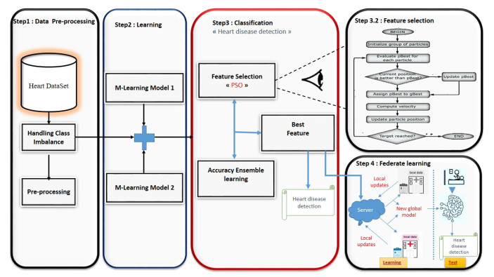
Predictive models for early identification of heart disease must be precise and efficient because it is a major worldwide health concern. To improve classification performance while protecting data privacy, this study investigated a combined method that uses ensemble learning, feature selection, and federated learning (FL). The ensemble-based approaches proved the most predictive after testing several different machine learning (ML) models, including random forests, the light gradient boosting machine, support vector machines, k-nearest neighbors, convolutional neural networks, and long short-term memory. We used particle swarm optimization (PSO) for feature selection, which optimized the most relevant features in conjunction with voting and stacking approaches to further increase the model's performance. In addition, federated learning was implemented to allow decentralized training while preserving sensitive medical data. The results highlight the effectiveness of combining these techniques in the detection of heart disease, providing a scalable and privacy-preserving solution for real-world healthcare applications. Two benchmark datasets were used to validate the proposed approach, ensuring the reliability and generalizability of the findings. Furthermore, we used four performance metrics, namely accuracy, precision, recall, and F1score, to evaluate the selected models. Finally, federated learning was included to handle privacy issues and guarantee safe access to private medical data. This distributed method allows model training without centralizing patient data, so it is compatible with strict data privacy rules. With up to 95% precision, our method shows a notable increase in prediction accuracy according to the testing results. This work offers a strong, scalable, and safe solution for the early identification of cardiovascular diseases by combining ensemble learning, feature selection, and federated learning, opening the way for more general uses in medical diagnostics.

References

[1]	S. Mendis, I. Graham, J. Narula, Addressing the global burden of cardiovascular diseases; need for scalable and sustainable frameworks, Glob. Heart, 17 (2022), 48. https://doi.org/10.5334/gh.1139 doi: 10.5334/gh.1139
[2]	A. Ala, A. Goli, Incorporating machine learning and optimization techniques for assigning patients to operating rooms by considering fairness policies, Eng. Appl. Artif. Intell., 136 (2024), 108980. https://doi.org/10.1016/j.engappai.2024.108980 doi: 10.1016/j.engappai.2024.108980
[3]	N. Chaithra, B. Madhu, Classification models on cardiovascular disease prediction using data mining techniques, J. Cardiovas. Dis. Diagn., 6 (2018), 10000348. https://doi.org/10.4172/2329-9517.1000348 doi: 10.4172/2329-9517.1000348
[4]	K. W. Johnson, J. T. Soto, B. S. Glicksberg, K. Shameer, R. Miotto, M. Ali, et al., Artificial intelligence in cardiology, JACC, 71 (2018), 2668–2679.
[5]	S. Kodati, R. Vivekanandam, Analysis of heart disease using in data mining tools orange and weka, Glob. J. Comput. Sci. Technol., 18 (2018), 16–22.
[6]	K. S. Shalet, V. Sabarinathan, V. Sugumaran, V. J. S. Kumar, Diagnosis of heart disease using decision tree and svm classifier, Int. J. Appl. Eng. Res., 10 (2015), 598–602.
[7]	K. Uyar, A. ˙Ilhan, Diagnosis of heart disease using genetic algorithm based trained recurrent fuzzy neural networks, Procedia Comput. Sci., 120 (2017), 588–593. https://doi.org/10.1016/j.procs.2017.11.283 doi: 10.1016/j.procs.2017.11.283
[8]	S. Khader Basha, D. Roja, S. Santhj Priya, L. Dalavi, S. Srinivas Vellela, V. Reddy, Coronary heart disease prediction and classification using hybrid machine learning algorithms, In: 2023 International Conference on Innovative Data Communication Technologies and Application (ICIDCA), IEEE, 2023. https://doi.org/10.1109/ICIDCA56705.2023.10099579
[9]	R. Jahed, O. Asser, A. Al-Mousa, Using personal key indicators and machine learning-based classifiers for the prediction of heart disease, In: 2023 International Conference on Smart Computing and Application (ICSCA), IEEE, 2023. https://doi.org/10.1109/ICSCA57840.2023.10087430
[10]	A. Rajdhan, A. Agarwal, M. Sai, D. Ravi, P. Ghuli, Heart disease prediction using machine learning, Int. J. Res. Technol., 9 (2020), 659–662.
[11]	C. Das, C. Das, M. Hossain, A. Rahman, H. Hossen, R. Hasan, Heart disease detection using ml, In: 2023 IEEE 13th Annual Computing and Communication Workshop and Conference (CCWC), IEEE, 2023. https://doi.org/10.1109/CCWC57344.2023.10099294
[12]	K. Pytlak, Indicators of heart disease (2022 update), 2022. Available from: https://www.kaggle.com/datasets/kamilpytlak/personal-key-indicators-of-heart-disease.
[13]	S. Chopra, N. Karla, R. Rani, Identification of cardiovascular disease using machine learning and ensemble learning, In: 2023 International Conference on Innovative Data Communication Technologies and Application (ICIDCA), IEEE, 2023. https://doi.org/10.1109/ICIDCA56705.2023.10099508
[14]	Z. Li, D. Zhou, L. Wan, J. Li, W. Mou, Heartbeat classification using deep residual convolutional neural network from 2-lead electrocardiogram, J. Electrocardiol., 58 (2020), 105–112. https://doi.org/10.1016/j.jelectrocard.2019.11.046 doi: 10.1016/j.jelectrocard.2019.11.046
[15]	L. B. Marinho, N. de MM Nascimento, J. W. M. Souza, M. V. Gurgel, P. P. R. Filho, V. H. C. de Albuquerque, A novel electrocardiogram feature extraction approach for cardiac arrhythmia classification, Future Gener. Comput. Syst., 97 (2019), 564–577. https://doi.org/10.1016/j.future.2019.03.025 doi: 10.1016/j.future.2019.03.025
[16]	S. Pandya, T. Gadekallu, P. Reddy, W. Wang, M. Alazab, Infusedheart: A novel knowledge-infused learning framework for diagnosis of cardiovascular events, IEEE Trans. Comput. Soc. Syst., 9 (2022), 1778–1788. https://doi.org/10.1109/TCSS.2022.3151643 doi: 10.1109/TCSS.2022.3151643
[17]	S. Mohan, C. Thirumalai, G. Srivastava, Effective heart disease prediction using hybrid machine learning techniques, IEEE Access, 7 (2019), 81542–81554. https://doi.org/10.1109/ACCESS.2019.2923707 doi: 10.1109/ACCESS.2019.2923707
[18]	R. Arun, N. Deepa, Heart disease prediction system using naive bayes, Int. J. Pure Appl. Math., 119 (2018), 3053–3065.
[19]	K. Prasanna, N. Challa, J. Nagaraju, Heart disease prediction using reinforcement learning technique, In: 2023 Third International Conference on Advances in Electrical, Computing, Communication and Sustainable Technologies (ICAECT), IEEE, 2023. https://doi.org/10.1109/ICAECT57570.2023.10118232
[20]	S. Bagavathy, V. Gomathy, S. S. Rani, M. Murugesan, K. Sujatha, M. K. Bhuvana, Early heart disease detection using data mining techniques with hadoop map reduce, Int. J. Pure Appl. Math., 119 (2018), 1915–1920.
[21]	A. Abdellatif, H. Abdellatef, J. Kanesan, C. O. Chow, J. H. Chuah, H. M. Gheni, An effective heart disease detection and severity level classification model using machine learning and hyperparameter optimization methods, IEEE Access, 10 (2022), 79974–79985. https://doi.org/10.1109/ACCESS.2022.3191669 doi: 10.1109/ACCESS.2022.3191669
[22]	H. Ramesh, R. Pathinarupothi, Performance analysis of machine learning algorithms to predict cardiovascular disease, In: 2023 IEEE 8th International Conference for Convergence in Technology (I2CT), IEEE, 2023. https://doi.org/10.1109/I2CT57861.2023.10126428
[23]	M. Shail, R. Sreeja, S. Zainab, P. S. Sowmya, T. Akshay, S. Sindhu, Improving accuracy of heart disease prediction through machine learning algorithms, In: 2023 International Conference on Innovative Data Communication Technologies and Application (ICIDCA), IEEE, 2023. https://doi.org/10.1109/ICIDCA56705.2023.10100244
[24]	L. Ali, A. Niamat, J. Khan, N. A. Golilarz, X. Xiong, A. Noor, et al., An optimized stacked support vector machines based expert system for the effective prediction of heart failure, IEEE Access, 7 (2019), 54007–54014. https://doi.org/10.1109/ACCESS.2019.2909969 doi: 10.1109/ACCESS.2019.2909969
[25]	T. Mahmud, A. Barua, M. Begum, E. Chakma, S. Das, N. Sharmen, An improved framework for reliable cardiovascular disease prediction using hybrid ensemble learning, In: 2023 International Conference on Electrical, Computer and Communication Engineering (ECCE), IEEE, 2023. https://doi.org/10.1109/ECCE57851.2023.10101564
[26]	B. Tama, S. Im, S. Lee, Improving an intelligent detection system for coronary heart disease using a two-tier classifier ensemble, Biomed Res. Int., 2020 (2020), 9816142. https://doi.org/10.1155/2020/9816142 doi: 10.1155/2020/9816142
[27]	O. Yildirim, A novel wavelet sequence based on a deep bidirectional lstm network model for ecg signal classification, Comput. Biol. Med., 96 (2018), 189–202. https://doi.org/10.1016/j.compbiomed.2018.03.016 doi: 10.1016/j.compbiomed.2018.03.016
[28]	N. Fitriyani, M. Syafrudin, G. Alfian, J. Rhee, Hdpm: An effective heart disease prediction model for a clinical decision support system, IEEE Access, 8 (2020), 133034–133050. https://doi.org/10.1109/ACCESS.2020.3010511 doi: 10.1109/ACCESS.2020.3010511
[29]	D. Shah, S. Patel, S. K. Bharti, Heart disease prediction using machine learning techniques, SN Comput. Sci., 1 (2020), 345. https://doi.org/10.1007/s42979-020-00365-y doi: 10.1007/s42979-020-00365-y
[30]	A. Jain, K. Kumar, R. Tiwari, N. Jain, V. Gautam, N. K. Trivedi, Machine learning-based detection of cardiovascular disease using classification and feature selection, In: 2023 IEEE 12th International Conference on Communication Systems and Network Technologies (CSNT), IEEE, 2023. https://doi.org/10.1109/CSNT57126.2023.10134672
[31]	A. Shukla, I. Khan, V. Sharma, M. Soni, S. Gupta, A. Kumar, A novel prediction system to diagnose heart disease, In: 2023 International Conference on Inventive Computation Technologies (ICICT), IEEE, 2023. https://doi.org/10.1109/ICICT57646.2023.10133988
[32]	G. Bathla, P. Singh, R. Singh, E. Cambria, R. Tiwari, Intelligent fake reviews detection based on aspect extraction and analysis using deep learning, Neural Comput. Appl., 34 (2022), 20213–20229. https://doi.org/10.1007/s00521-022-07531-8 doi: 10.1007/s00521-022-07531-8
[33]	G. Varshini, A. Ramya, C. Sravya, V. Kumar, B. K. Shukla, Improving heart disease prediction of classifiers with data transformation using pca and relief feature selection, In: 2023 Second International Conference on Electronics and Renewable Systems (ICEARS), IEEE, 2023. https://doi.org/10.1109/ICEARS56392.2023.10085401
[34]	G. Saranya, A. Pravin, A comprehensive study on disease risk predictions in machine learning, Int. J. Elect. Comput. Eng., 10 (2020), 4217–4225. https://doi.org/10.11591/ijece.v10i4.pp4217-4225 doi: 10.11591/ijece.v10i4.pp4217-4225
[35]	M. Singh, L. M. Martins, P. Joanis, V. K. Mago, Building a cardiovascular disease predictive model using structural equation model & fuzzy cognitive map, In: International Conference on Fuzzy Systems (FUZZ), IEEE, 2016, 1377–1382. https://doi.org/10.1109/FUZZ-IEEE.2016.7737850
[36]	K. Sen, B. Verma, Heart disease prediction using a soft voting ensemble of gradient boosting models, randomforest, and gaussian naive bayes, In: 2023 4th International Conference for Emerging Technology (INCET), IEEE, 2023. https://doi.org/10.1109/INCET57972.2023.10170399
[37]	K. Gola, S. Arya, Satin bowerbird optimization-based classification model for heart disease prediction using deep learning in e-healthcare, In: 2023 IEEE/ACM 23rd International Symposium on Cluster, Cloud and Internet Computing Workshops (CCGridW), IEEE, 2023. https://doi.org/10.1109/CCGridW59191.2023.00063
[38]	J. Patel, T. Upadhyay, S. Patel, Heart disease prediction using machine learning and data mining technique, IJCSC, 7 (2015), 129–137.
[39]	A. Pandita, S. Yadav, S. Vashisht, A. Tyagi, Review paper on prediction of heart disease using machine learning algorithms, Int. J. Res. Appl. Sci. Eng. Technol., 9 (2021).
[40]	A. Akella, S. Akella, Machine learning algorithms for predicting coronary artery disease: efforts toward an open-source solution, Future Sci. OA, 7 (2021), FSO698.
[41]	A. Ala, V. Simic, D. Pamucar, N. Bacanin, Enhancing patient information performance in internet of things-based smart healthcare system: Hybrid artificial intelligence and optimization approaches, Eng. Appl. Artif. Intell., 131 (2024), 107889. https://doi.org/10.1016/j.engappai.2024.107889 doi: 10.1016/j.engappai.2024.107889
[42]	M. Nazari, H. Emami, R. Rabiei, A. Hosseini, S. Rahmatizadeh, Detection of cardiovascular diseases using data mining approaches: Application of an ensemble-based model, Cogn. Comput., 16 (2024), 2264–-2278. https://doi.org/10.1007/s12559-024-10306-z doi: 10.1007/s12559-024-10306-z
[43]	S. Mokeddem, B. Atmani, M. Mokaddem, Supervised feature selection for diagnosis of coronary artery disease based on genetic algorithm, preprint paper, 2013. https://doi.org/10.48550/arXiv.1305.6046
[44]	J. C. T. Arroyo, A. J. P. Delima, An optimized neural network using genetic algorithm for cardiovascular disease prediction, J. Adv. Inf. Technol., 13 (2022), 95–99. https://doi.org/10.12720/jait.13.1.95-99 doi: 10.12720/jait.13.1.95-99

Reader Comments

Your name:*

Email:*
© 2025 the Author(s), licensee AIMS Press. This is an open access article distributed under the terms of the Creative Commons Attribution License (http://creativecommons.org/licenses/by/4.0)