Intuitionistic fuzzy-based TOPSIS method for multi-criterion optimization problem: a novel compromise methodology

Ya Qin; Rizk M. Rizk-Allah; Harish Garg; Aboul Ella Hassanien; Václav Snášel; Ya Qin; Rizk M. Rizk-Allah; Harish Garg; Aboul Ella Hassanien; Václav Snášel

doi:10.3934/math.2023860

AIMS Mathematics

2023, Volume 8, Issue 7: 16825-16845. doi: 10.3934/math.2023860

Previous Article Next Article

Research article

Intuitionistic fuzzy-based TOPSIS method for multi-criterion optimization problem: a novel compromise methodology

1.
School of Mathematics and Information Sciences, Numerical Simulation Key Laboratory of Sichuan Provincial Universities, Neijiang Normal University, Neijiang 641000, Sichuan, China
2.
Department of Basic Engineering Science, Faculty of Engineering, Menoufia University, Shebin El-Kom 32511, Egypt
3.
Faculty of Electrical Engineering and Computer Science, VŠB-Technical University of Ostrava, Poruba-Ostrava 70800, Czech Republic
4.
School of Mathematics, Thapar Institute of Engineering & Technology (Deemed University), Patiala 147004, Punjab, India
5.
Applied Science Research Center, Applied Science Private University, Amman 11931, Jordan
6.
Department of Mathematics, Graphic Era Deemed to be University, Dehradun 248002, Uttarakhand, India
7.
College of Technical Engineering, The Islamic University, Najaf, Iraq
8.
Faculty of Computers and AI, Cairo University, Egypt

Received: 16 February 2023 Revised: 24 April 2023 Accepted: 25 April 2023 Published: 15 May 2023
MSC : 03E72, 08A72, 54A40

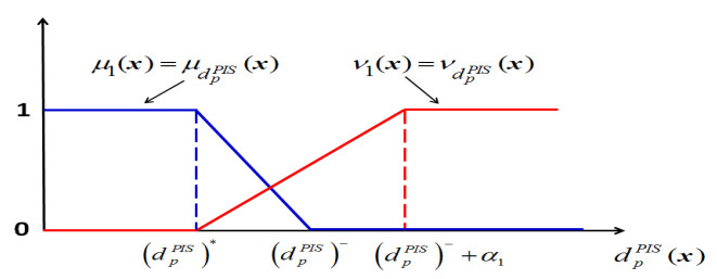
The decision-making process is characterized by some doubt or hesitation due to the existence of uncertainty among some objectives or criteria. In this sense, it is quite difficult for decision maker(s) to reach the precise/exact solutions for these objectives. In this study, a novel approach based on integrating the technique for order preference by similarity to ideal solution (TOPSIS) with the intuitionistic fuzzy set (IFS), named TOPSIS-IFS, for solving a multi-criterion optimization problem (MCOP) is proposed. In this context, the TOPSIS-IFS operates with two phases to reach the best compromise solution (BCS). First, the TOPSIS approach aims to characterize the conflicting natures among objectives by reducing these objectives into only two objectives. Second, IFS is incorporated to obtain the solution model under the concept of indeterminacy degree by defining two membership functions for each objective (i.e., satisfaction degree, dissatisfaction degree). The IFS can provide an effective framework that reflects the reality contained in any decision-making process. The proposed TOPSIS-IFS approach is validated by carrying out an illustrative example. The obtained solution by the approach is superior to those existing in the literature. Also, the TOPSIS-IFS approach has been investigated through solving the multi-objective transportation problem (MOTP) as a practical problem. Furthermore, impacts of IFS parameters are analyzed based on Taguchi method to demonstrate their effects on the BCS. Finally, this integration depicts a new philosophy in the mathematical programming field due to its interesting principles.
- multi-criterion optimization,
- intuitionistic fuzzy,
- TOPSIS,
- compromise solution,
- Taguchi method
Citation: Ya Qin, Rizk M. Rizk-Allah, Harish Garg, Aboul Ella Hassanien, Václav Snášel. Intuitionistic fuzzy-based TOPSIS method for multi-criterion optimization problem: a novel compromise methodology[J]. AIMS Mathematics, 2023, 8(7): 16825-16845. doi: 10.3934/math.2023860

Related Papers:

Abstract

The decision-making process is characterized by some doubt or hesitation due to the existence of uncertainty among some objectives or criteria. In this sense, it is quite difficult for decision maker(s) to reach the precise/exact solutions for these objectives. In this study, a novel approach based on integrating the technique for order preference by similarity to ideal solution (TOPSIS) with the intuitionistic fuzzy set (IFS), named TOPSIS-IFS, for solving a multi-criterion optimization problem (MCOP) is proposed. In this context, the TOPSIS-IFS operates with two phases to reach the best compromise solution (BCS). First, the TOPSIS approach aims to characterize the conflicting natures among objectives by reducing these objectives into only two objectives. Second, IFS is incorporated to obtain the solution model under the concept of indeterminacy degree by defining two membership functions for each objective (i.e., satisfaction degree, dissatisfaction degree). The IFS can provide an effective framework that reflects the reality contained in any decision-making process. The proposed TOPSIS-IFS approach is validated by carrying out an illustrative example. The obtained solution by the approach is superior to those existing in the literature. Also, the TOPSIS-IFS approach has been investigated through solving the multi-objective transportation problem (MOTP) as a practical problem. Furthermore, impacts of IFS parameters are analyzed based on Taguchi method to demonstrate their effects on the BCS. Finally, this integration depicts a new philosophy in the mathematical programming field due to its interesting principles.

References

[1]	K. T. Attanassov, Intuitionistic fuzzy sets, Fuzzy Set. Syst., 20 (1986), 87–96. https://doi.org/10.1016/S0165-0114(86)80034-3 doi: 10.1016/S0165-0114(86)80034-3
[2]	R. E. Bellman, L. A. Zadeh, Decision making in a fuzzy environment, Manage. Sci., 17 (1970), 141–164. https://doi.org/10.1287/mnsc.17.4.B141 doi: 10.1287/mnsc.17.4.B141
[3]	P. P. Angelov, Optimization in an intuitionistic fuzzy environment, Fuzzy Set. Syst., 86 (1997), 299–306. https://doi.org/10.1016/S0165-0114(96)00009-7 doi: 10.1016/S0165-0114(96)00009-7
[4]	S. Dey, T. K. Roy, Multi-objective structural optimization using fuzzy and intuitionistic fuzzy optimization technique, International Journal of Intelligent Systems and Applications, 5 (2015), 57–65. https://doi.org/10.5815/ijisa.2015.05.08 doi: 10.5815/ijisa.2015.05.08
[5]	B. Jana, T. K. Roy, Multi-objective intuitionistic fuzzy linear programming and its application in transportation model, Notes on Intuitionistic Fuzzy Sets, 13 (2007), 34–51.
[6]	O. Bahri, E. Talbi, N. B. Amor, A generic fuzzy approach for multi-objective optimization under uncertainty, Swarm Evol. Comput., 40 (2018), 166–183. https://doi.org/10.1016/j.swevo.2018.02.002 doi: 10.1016/j.swevo.2018.02.002
[7]	C. L. Hwang, K. Yoon, Multiple attribute decision making: methods and applications, Heidelberg: Springer, 1981. https://doi.org/10.1007/978-3-642-48318-9
[8]	C. H. Yeh, The selection of multiattribute decision making methods for scholarship student selection, Int. J. Select. Assess., 11 (2003), 289–296. https://doi.org/10.1111/j.0965-075X.2003.00252.x doi: 10.1111/j.0965-075X.2003.00252.x
[9]	E. K. Zavadskas, A. Mardani, Z. Turskis, A. Jusoh, K. M. Nor, Development of TOPSIS method to solve complicated decision-making problems-an overview on developments from 2000 to 2015, Int. J. Inf. Tech. Decis., 15 (2016), 645–682. https://doi.org/10.1142/S0219622016300019 doi: 10.1142/S0219622016300019
[10]	V. P. Agrawal, V. Kohli, S. Gupta, Computer aided robot selection: the 'multiple attribute decision making' approach, Int. J. Prod. Res., 29 (1991), 1629–1644. https://doi.org/10.1080/00207549108948036 doi: 10.1080/00207549108948036
[11]	C. Parkan, M. L. Wu, Decision-making and performance measurement models with applications to robot selection, Comput. Ind. Eng., 36 (1999), 503–523. https://doi.org/10.1016/S0360-8352(99)00146-1 doi: 10.1016/S0360-8352(99)00146-1
[12]	E. Akgul, M. I. Bahtiyari, E. K. Aydoğan, H. Benli, Use of TOPSIS method for designing different textile products in coloration via natural source madder, J. Nat. Fivers, 19 (2021), 8993–9008. https://doi.org/10.1080/15440478.2021.1982106 doi: 10.1080/15440478.2021.1982106
[13]	M. Tavana, A. Hatami-Marbini, A group AHP-TOPSIS framework for human spaceflight mission planning at NASA, Expert Syst. Appl., 38 (2011), 13588–13603. https://doi.org/10.1016/j.eswa.2011.04.108 doi: 10.1016/j.eswa.2011.04.108
[14]	R. M. Rizk-Allah, E. A. Hagag, A. A. El-Fergany, Chaos-enhanced multi-objective tunicate swarm algorithm for economic-emission load dispatch problem, Soft Comput., 27 (2023), 5721–5739. https://doi.org/10.1007/s00500-022-07794-2 doi: 10.1007/s00500-022-07794-2
[15]	R. M. Rizk-Allah, M. A. Abo-Sinna, A. E. Hassanien, Intuitionistic fuzzy sets and dynamic programming for multi-objective non-linear programming problems, Int. J. Fuzzy Syst., 23 (2021), 334–352. https://doi.org/10.1007/s40815-020-00973-z doi: 10.1007/s40815-020-00973-z
[16]	R. M. Rizk-Allah, M. A. Abo-Sinna, A comparative study of two optimization approaches for solving bi-level multi-objective linear fractional programming problem, OPSEARCH, 58 (2021), 374–402. https://doi.org/10.1007/s12597-020-00486-1 doi: 10.1007/s12597-020-00486-1
[17]	D. Chakraborty, D. K. Jana, T. K. Roy, Arithmetic operations on generalized intuitionistic fuzzy number and its applications to transportation problem, OPSEARCH, 52 (2015), 431–471. https://doi.org/10.1007/s12597-014-0194-1 doi: 10.1007/s12597-014-0194-1
[18]	D. Chakraborty, D. K. Jana, T. K. Roy, A new approach to solve multi-objective multi- choice multi-item Atanassov's intuitionistic fuzzy transportation problem using chance operator, J. Intell. Fuzzy Syst., 28 (2015), 843–865. doi: 10.3233/IFS-141366
[19]	J. Razmi, E. Jafarian, S. H. Amin, An intuitionistic fuzzy goal programming approach for finding pareto-optimal solutions to multi-objective programming problems, Expert Syst. Appl., 65 (2016), 181–193. https://doi.org/10.1016/j.eswa.2016.08.048 doi: 10.1016/j.eswa.2016.08.048
[20]	S. Pramanik, T. K. Roy, An intuitionistic fuzzy goal programming approach to vector optimization problem, Notes on Intuitionistic Fuzzy Sets, 11 (2005), 1–14.
[21]	S. Chakrabortty, M. Pal, P. K. Nayak, Intuitionistic fuzzy optimization technique for Pareto optimal solution of manufacturing inventory models with shortages, Eur. J. Oper. Res., 228 (2013), 381–387. https://doi.org/10.1016/j.ejor.2013.01.046 doi: 10.1016/j.ejor.2013.01.046
[22]	H. Garg, M. Rani, An approach for reliability analysis of industrial systems using PSO and IFS technique, ISA T., 52 (2013), 701–710. https://doi.org/10.1016/j.isatra.2013.06.010 doi: 10.1016/j.isatra.2013.06.010
[23]	A. Yildiz, A. F. Guneri, C. Ozkan, E. Ayyildiz, A. Taskin, An integrated interval-valued intuitionistic fuzzy AHP-TOPSIS methodology to determine the safest route for cash in transit operations: a real case in Istanbul, Neural. Comput. & Applic., 34 (2022), 15673–15688. https://doi.org/10.1007/s00521-022-07236-y doi: 10.1007/s00521-022-07236-y
[24]	S. K. Das, N. Dey, R. G. Crespo, E. Herrera-Viedma, A non-linear multi-objective technique for hybrid peer-to-peer communication, Inform. Sciences, 629 (2023), 413–439. https://doi.org/10.1016/j.ins.2023.01.117 doi: 10.1016/j.ins.2023.01.117
[25]	R. M. Rizk-Allah, M. A. Abo-Sinna, Integrating reference point, Kuhn-Tucker conditions and neural network approach for multi-objective and multi-level programming problems, OPSEARCH, 54 (2017), 663–683. https://doi.org/10.1007/s12597-017-0299-4 doi: 10.1007/s12597-017-0299-4
[26]	N. Karimi, M. R. Feylizadeh, K. Govindan, M. Bagherpour, Fuzzy multi-objective programming: a systematic literature review, Expert Syst. Appl., 196 (2022), 116663. https://doi.org/10.1016/j.eswa.2022.116663 doi: 10.1016/j.eswa.2022.116663
[27]	R. M. Rizk-Allah, R. A. El-Sehiemy, S. Deb, G. G. Wang, A novel fruit fly framework for multi-objective shape design of tubular linear synchronous motor, J. Supercomput., 73 (2017), 1235–1256. https://doi.org/10.1007/s11227-016-1806-8 doi: 10.1007/s11227-016-1806-8
[28]	R. A. El-Sehiemy, R. M. Rizk-Allah, A. F. Attia, Assessment of hurricane versus sine‐cosine optimization algorithms for economic/ecological emissions load dispatch problem, Int. T. Electr. Energy, 29 (2019), e2716. https://doi.org/10.1002/etep.2716 doi: 10.1002/etep.2716
[29]	R. M. Rizk-Allah, A. E. Hassanien, D. Oliva, An enhanced sitting–sizing scheme for shunt capacitors in radial distribution systems using improved atom search optimization, Neural Comput. & Applic., 32 (2020), 13971–13999. https://doi.org/10.1007/s00521-020-04799-6 doi: 10.1007/s00521-020-04799-6
[30]	K. Miettinen, Nonlinear multiobjective optimization, New York: Springer, 1998. https://doi.org/10.1007/978-1-4615-5563-6
[31]	Y. J. Lai, T. J. Liu, C. L. Hwang, TOPSIS for MODM, Eur. J. Oper. Res., 76 (1994), 486–500. https://doi.org/10.1016/0377-2217(94)90282-8 doi: 10.1016/0377-2217(94)90282-8
[32]	L. A. Zadeh, Fuzzy sets, Information and Control, 8 (1965), 338–353. https://doi.org/10.1016/S0019-9958(65)90241-X doi: 10.1016/S0019-9958(65)90241-X
[33]	A. Kaufmann, M. M. Gupta, Introduction to fuzzy arithmetic, New York: Van Nostrand, 1991.
[34]	M. A. Abo-Sinna, A. H. Amer, Extensions of TOPSIS for multi-objective large-scale nonlinear programming problems, Appl. Math. Comput., 162 (2005), 243–256. https://doi.org/10.1016/j.amc.2003.12.087 doi: 10.1016/j.amc.2003.12.087
[35]	P. Singh, S. Kumari, S. Singh, Fuzzy efficient interactive goal programming approach for multi-objective transportation problems, Int. J. Appl. Comput. Math., 3 (2017), 505–525. https://doi.org/10.1007/s40819-016-0155-x doi: 10.1007/s40819-016-0155-x
[36]	D. C. Montgomery, Design and analysis of experiments, Arizona: John Wiley & Sons, 2005.
[37]	R. M. Rizk-Allah, R. A. El-Sehiemy, G. G. Wang, A novel parallel hurricane optimization algorithm for secure emission/economic load dispatch solution, Appl. Soft Comput., 63 (2018), 206–222. https://doi.org/10.1016/j.asoc.2017.12.002 doi: 10.1016/j.asoc.2017.12.002
[38]	S. Boopathi, Experimental investigation and parameter analysis of LPG refrigeration system using Taguchi method, SN Appl. Sci., 1 (2019), 892. https://doi.org/10.1007/s42452-019-0925-2 doi: 10.1007/s42452-019-0925-2
[39]	N. S. Patel, P. L. Parihar, J. S. Makwana, Parametric optimization to improve the machining process by using Taguchi method: a review, Materials Today: Proceedings, 47 (2021), 2709–2714. https://doi.org/10.1016/j.matpr.2021.03.005 doi: 10.1016/j.matpr.2021.03.005
[40]	R. M. Rizk-Allah, A. E. Hassanien, D. Song, Chaos-opposition-enhanced slime mould algorithm for minimizing the cost of energy for the wind turbines on high-altitude sites, ISA T., 121 (2022), 191–205. https://doi.org/10.1016/j.isatra.2021.04.011 doi: 10.1016/j.isatra.2021.04.011
[41]	Y. Kuo, T. Yang, G. W. Huang, The use of a grey-based Taguchi method for optimizing multi-response simulation problems, Eng. Optimiz., 40 (2008), 517–528. https://doi.org/10.1080/03052150701857645 doi: 10.1080/03052150701857645
[42]	X. Li, Y. Sun, Stock intelligent investment strategy based on support vector machine parameter optimization algorithm, Neural Comput. & Applic., 32 (2020), 1765–1775. https://doi.org/10.1007/s00521-019-04566-2 doi: 10.1007/s00521-019-04566-2
[43]	B. Cao, M. Li, X. Liu, J. Zhao, W. Cao, Z. Lv, Many-objective deployment optimization for a Drone-Assisted camera network, IEEE T. Netw. Sci. Eng., 8 (2021), 2756–2764. https://doi.org/10.1109/TNSE.2021.3057915 doi: 10.1109/TNSE.2021.3057915
[44]	B. Cao, S. Fan, J. Zhao, S. Tian, Z. Zheng, Y. Yan, et al., Large-scale many-objective deployment optimization of edge servers, IEEE T. Intell. Transp., 99 (2021), 1–9. https://doi.org/10.1109/TITS.2021.3059455 doi: 10.1109/TITS.2021.3059455
[45]	S. G. Li, Efficient algorithms for scheduling equal-length jobs with processing set restrictions on uniform parallel batch machines, Math. Biosci. Eng., 19 (2022), 10731–10740. https://doi.org/10.3934/mbe.2022502 doi: 10.3934/mbe.2022502

Reader Comments

Your name:*

Email:*
© 2023 the Author(s), licensee AIMS Press. This is an open access article distributed under the terms of the Creative Commons Attribution License (http://creativecommons.org/licenses/by/4.0)