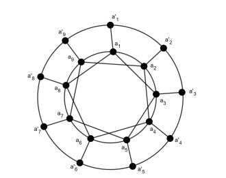
For a connected network Γ, the distance between any two vertices is the length of the shortest path between them. A vertex c in a connected network is said to resolve an edge e if the distances of c from its endpoints are unequal. The collection of all the vertices which resolve an edge is called the local resolving neighborhood set of this edge. A local resolving function is a real-valued function is defend as η:V(Γ)→[0,1] such that η(Rx(e))≥1 for each edge e∈E(Γ), where Rx(e) represents the local resolving neighborhood set of a connected network. Thus the local fractional metric dimension is defined as dimLF(Γ)=min{|η|:ηistheminimallocalresolvingfunctionofΓ}, where |η|=∑a∈Rx(e)η(a). In this manuscript, we have established sharp bounds of the local fractional metric dimension of different types of modified prism networks and it is also proved that local fractional metric dimension remains bounded when the order of these networks approaches to infinity.
Citation: Ahmed Alamer, Hassan Zafar, Muhammad Javaid. Study of modified prism networks via fractional metric dimension[J]. AIMS Mathematics, 2023, 8(5): 10864-10886. doi: 10.3934/math.2023551
[1] | Ridha Dida, Hamid Boulares, Bahaaeldin Abdalla, Manar A. Alqudah, Thabet Abdeljawad . On positive solutions of fractional pantograph equations within function-dependent kernel Caputo derivatives. AIMS Mathematics, 2023, 8(10): 23032-23045. doi: 10.3934/math.20231172 |
[2] | Choukri Derbazi, Zidane Baitiche, Mohammed S. Abdo, Thabet Abdeljawad . Qualitative analysis of fractional relaxation equation and coupled system with Ψ-Caputo fractional derivative in Banach spaces. AIMS Mathematics, 2021, 6(3): 2486-2509. doi: 10.3934/math.2021151 |
[3] | Kishor D. Kucche, Sagar T. Sutar, Kottakkaran Sooppy Nisar . Analysis of nonlinear implicit fractional differential equations with the Atangana-Baleanu derivative via measure of non-compactness. AIMS Mathematics, 2024, 9(10): 27058-27079. doi: 10.3934/math.20241316 |
[4] | Lahcene Rabhi, Mohammed Al Horani, Roshdi Khalil . Existence results of mild solutions for nonlocal fractional delay integro-differential evolution equations via Caputo conformable fractional derivative. AIMS Mathematics, 2022, 7(7): 11614-11634. doi: 10.3934/math.2022647 |
[5] | Abdelatif Boutiara, Mohammed S. Abdo, Mohammed A. Almalahi, Kamal Shah, Bahaaeldin Abdalla, Thabet Abdeljawad . Study of Sturm-Liouville boundary value problems with p -Laplacian by using generalized form of fractional order derivative. AIMS Mathematics, 2022, 7(10): 18360-18376. doi: 10.3934/math.20221011 |
[6] | Mohamed I. Abbas, Maria Alessandra Ragusa . Nonlinear fractional differential inclusions with non-singular Mittag-Leffler kernel. AIMS Mathematics, 2022, 7(11): 20328-20340. doi: 10.3934/math.20221113 |
[7] | Cuiying Li, Rui Wu, Ranzhuo Ma . Existence of solutions for Caputo fractional iterative equations under several boundary value conditions. AIMS Mathematics, 2023, 8(1): 317-339. doi: 10.3934/math.2023015 |
[8] | Ahmed M. A. El-Sayed, Wagdy G. El-Sayed, Kheria M. O. Msaik, Hanaa R. Ebead . Riemann-Liouville fractional-order pantograph differential equation constrained by nonlocal and weighted pantograph integral equations. AIMS Mathematics, 2025, 10(3): 4970-4991. doi: 10.3934/math.2025228 |
[9] | Weerawat Sudsutad, Chatthai Thaiprayoon, Aphirak Aphithana, Jutarat Kongson, Weerapan Sae-dan . Qualitative results and numerical approximations of the (k,ψ)-Caputo proportional fractional differential equations and applications to blood alcohol levels model. AIMS Mathematics, 2024, 9(12): 34013-34041. doi: 10.3934/math.20241622 |
[10] | Kulandhaivel Karthikeyan, Palanisamy Raja Sekar, Panjaiyan Karthikeyan, Anoop Kumar, Thongchai Botmart, Wajaree Weera . A study on controllability for Hilfer fractional differential equations with impulsive delay conditions. AIMS Mathematics, 2023, 8(2): 4202-4219. doi: 10.3934/math.2023209 |
For a connected network Γ, the distance between any two vertices is the length of the shortest path between them. A vertex c in a connected network is said to resolve an edge e if the distances of c from its endpoints are unequal. The collection of all the vertices which resolve an edge is called the local resolving neighborhood set of this edge. A local resolving function is a real-valued function is defend as η:V(Γ)→[0,1] such that η(Rx(e))≥1 for each edge e∈E(Γ), where Rx(e) represents the local resolving neighborhood set of a connected network. Thus the local fractional metric dimension is defined as dimLF(Γ)=min{|η|:ηistheminimallocalresolvingfunctionofΓ}, where |η|=∑a∈Rx(e)η(a). In this manuscript, we have established sharp bounds of the local fractional metric dimension of different types of modified prism networks and it is also proved that local fractional metric dimension remains bounded when the order of these networks approaches to infinity.
As we know today, the role of fractional operators or, rather, fractional calculus, in the study and investigation of natural phenomena is undeniable, if not irreplaceable. Certainly, the most important reason for the stunning growth of fractional calculus in the last decade can be seen in its ability and application in modeling biological [1,2,3,4] and physical [5,6,7,8,9] phenomena. As one of the most prominent features of fractional operators, we can mention their non-locality. Based on the available results and evidence, modeling by ordinary calculus is not capable of describing the real behavior of phenomena and is often associated with the error of estimating the phenomenon [10]. Researchers in the fields of science and engineering have different approaches to the non-local character of fractional calculus. Physicists' approach to this issue has led to interesting modeling schemes for physical phenomena such as heat flow, hereditary polarization in dielectrics, viscoelasticity and so on [11]. Such phenomena have been modeled with equations which are influenced by the past values of one or more variables, and they are called equations with memory in the literature. Mathematicians have also provided the basis for extending the existing models for different fields by generalizing the fractional operators. The most basic fractional operator is the derivative given by Riemann and Liouville (namely, the Riemann-Liouville derivative). With the publication of a book in 1999, Podlubny may have contributed the most to the systematic presentation of the theory of fractional operators [12]. Taking ideas from his works, we have witnessed the introduction of various operators, such as the Caputo, Hilfer, Atangana-Baleanu, Hadamard, fractal fractional, Caputo-Fabrizio, fractional q-derivative and (p,q)-derivative operators, etc., in the last two decades. For get more information about these contributions, one can refer to [13,14,15,16,17,18,19,20,21]. There is a certain type of kernel dependency included in all of those definitions. That is, we can consider a general operator from which fractional integral and derivative operators can be extracted by selecting specific kernels [22,23,24].
One of the most recent generalizations of fractional operators is related to the work of the Portuguese mathematician Ricardo Almeida. In 2017, he presented a new definition of the Caputo derivative, namely, ψ-Caputo, with respect to another non-decreasing function, such as ψ [25]. In his new model, the Riemann-Liouville and Hadamard fractional operators are obtained by choosing ψ(κ)=κ and ψ(κ)=lnκ. A year later, he and colleagues investigated the existence and uniqueness of the solution for an initial value problem with his new fractional operator, and, using it, he presented a model for the growth of the world population and the gross domestic product growth rate in the USA [26]. In 2019, Abdo et al. studied the existence and uniqueness of the solution for initial and boundary value problems with the ψ-Caputo derivative [27,28]. In 2020, Wahash et al. investigated fractional differential equations with singularities by applying the ψ-Caputo operator using the Picard iteration method [29]. Voyiadjis and Sumelka used this new type of fractional operator to provide an important model of brain damage in the framework of anisotropic hyperelasticity [30]. Also, Ahmed et al, presented a model for thermostats by using this fractional operator [31]. For more contributions that include this new fractional operator, the reader can see [32,33,34,35]. Here, we are going to present a model for the pantograph equation using the ψ-Caputo fractional operator; however, we will continue this section with a discussion about the pantograph.
Considering the issues raised and the potential in fractional operators, it is not far from expected that we also want to present a model for one of the most important and widely used equations in applied sciences, that is, the pantograph equation. Usually, the pantograph reminds us of a device that is installed on the top of the roof of electric buses. The pantograph problem was first raised by Mr. E. A. Cardwell of the British Railways Technical Center, at the Conference on Applications of Differential Equations in 1969. Ockendon and Tayler, in 1971, presented a mathematical model for Pantograph motion [36]. Today, the pantograph in electric trains is a tool that converts the electric current from direct to alternating current [37]. The pantograph differential equation is widely used in various fields, including number theory, quantum mechanics, statistics and electrodynamics [38,39]. Many researchers have investigated the pantograph equation from different aspects. For example, numerical solutions via Chebyshev polynomials are presented in [40], the existence of mild solutions to pantograph equations are investigated in [41], the stability of solutions was studied in [42] and a coupled system of pantograph problems using sequential fractional derivatives was examined in [43]. To access more information, see [44,45,46,47,48].
The standard mode of the pantograph equation is formulated as follows:
{w′(κ)=c1w(κ)+c2w(εκ),0≤κ≤K,w(0)=w0, |
such that 0<ε<1 [49]. The fractional case of the pantograph equation investigated by Balachandran et al. involving the Caputo operator is as follows:
{CDηw(κ)=h(κ,w(κ),w(εκ)),0≤κ≤K,w(0)=w0, |
where 0<ȷ and ε<1 [49].
To the best of our knowledge, topological degree theory for condensing maps has not been applied to nonlinear pantograph differential equations with ψ-Caputo fractional derivatives under nonlocal boundary conditions. Therefore, inspired by the history mentioned above and previous works, in this paper, we investigate the existence of solutions for the following nonlinear fractional pantograph differential equation:
{CDη,ψw(κ)=h(κ,w(κ),w(εκ)),κ∈K=[0,K],w′(0)=0,w(0)+χ(w)=w0, | (1.1) |
where CDη,ψ is the ψ-Caputo fractional derivative of order η∈(1,2), ε∈(0,1), K>0, h∈C(K×R2,R), w0∈R and χ is the nonlocal term that satisfies some given conditions. The importance of the nonlocal condition, which is better than the classical initial condition, is explained in [50]. Furthermore, in recent research in 2021, Sabatier and Farges showed, by designing some problems and numerical analysis, that the use of fractional derivatives is problematic in some fractional models [51]. According to the above topics, in this work, we also considered the boundary conditions as nonlocal, although the authors, as mentioned have other works with fractional initial conditions applied in this matter [43].
The rest of the paper is structured as follows. In Section 2, we state what we need from fractional calculus and topological degree theory as preliminaries to prove our main results. In Section 3, we first introduce three hypotheses, prove four auxiliary lemmas and prove the existence of solutions for the pantograph equation given by (1.1). In Section 4, we present examples with numerical and graphical simulations to validate our results. The last section concludes this paper.
This section deals with some preliminaries and notations which are used throughout this paper. For more details, we refer the reader to [25].
Definition 2.1. [26] Assume that w is an integrable function on K=[0,K], and that ψ∈Cn(K,R), where ∀κ∈K, ψ′(κ)>0. Then, the ψ-Riemann-Liouville (ψ-RL) integral and derivative of w of fractional order ȷ is expressed as follows:
Iȷ,ψw(κ)=1Γ(ȷ)∫κ0ψ′(p)(ψ(κ)−ψ(p))ȷ−1w(p)dp, |
and
Dȷ,ψw(κ)=1Γ(ȷ−n)(1ψ′(κ)ddκ)n∫κ0ψ′(p)(ψ(κ)−ψ(p))n−ȷ−1w(p)dp=(1ψ′(κ)ddκ)nIn−ȷ,ψw(κ), |
where n=[ȷ]+1.
Definition 2.2. [26] Suppose that w∈Cn−1(K,R) and ψ∈Cn(K,R) such that ∀κ∈K, ψ′(κ)>0. Then, the Ψ-Caputo operator of fractional order ȷ is formulated as follows:
CDȷ,ψw(κ)=1Γ(n−ȷ)∫κ0ψ′(p)(ψ(κ)−ψ(p))n−ȷ−1w[n]ψ(p)dp, | (2.1) |
where
w[n]ψ(p)=(1ψ′(p)ddp)nw(p),n=[ȷ]+1. |
Remark 2.1. It is obvious that, with correct placement, namely, ψ(κ)=κ and ψ(κ)=ln(κ), in (2.1), the Caputo and Caputo-Hadamard derivatives can be reached.
Remark 2.2. If 0<ȷ<1, then we have
CDȷ,ψw(κ)=1Γ(1−ȷ)(1ψ′(p)ddp)1∫κ0(ψ(κ)−Ψ(p))−ȷw(p)dp. |
Theorem 2.1. [26] If ȷ>0 and w∈Cn−1(K,R), then the following assertions hold:
1) CDȷ,ψIȷ,ψw(κ)=w(κ).
2) Iȷ,ψCDȷ,ψw(κ)=w(κ)−∑n−1i=0w[i]ψ(0)i!(ψ(κ)−ψ(0))i.
Theorem 2.2. [26] Let μ>ν>0 and κ∈K; then, we have the following:
1) Iμ,ψ(ψ(κ)−ψ(0))ν−1=Γ(ν)Γ(μ+ν)(ψ(t)−ψ(0))μ+ν−1.
2) Dμ,ψ(ψ(t)−ψ(0))ν−1=Γ(ν)Γ(ν−μ)(ψ(κ)−ψ(0))ν−μ−1.
3) Dμ,ψ(ψ(κ)−ψ(0))p=0, ∀p<n∈N.
Definition 2.3. [52] Suppose that X is a Banach space and BX={Y⊂X:Y≠∅,Yis bounded}. The function ρ : BX→[0,+∞) is called the Kuratowski measure of non-compactness and defined as follows:
ρ(Y)=inf{r>0:Yadmits a finite cover by sets of diameter ≤r}. |
Theorem 2.3. [52] The measure ρ defined above, namely, Definition 2.3, applies to the following properties.
(1) ρ(Y)=0 iff Y is relativity compact.
(2) ρ(aY)=|a|ρ(Y),a∈R.
(3) ρ(Y1+Y2)≤ρ(Y1)+ρ(Y2).
(4) If Y1⊂Y2, then ρ(Y1)≤ρ(Y2).
(5) ρ(Y1∪Y2)=max{ρ(Y1), ρ(Y2)}.
(6) ρ(Y)=ρ(¯Y)=ρ(convY), where ¯Y and convY denote the closure and convex hull of Y, respectively.
Definition 2.4. [52] Assume that the function Θ:Y⊂X→X is a continuous and bounded map. The function Θ is called ρ-Lipschitz if ∃ℓ≥0, given that
ρ(Θ(Y∗))≤ℓρ(Y∗),Y∗⊂Y. |
Definition 2.5. [52] The function Θ, which is defined in Definition 2.4 is called ρ-condensing if, for every bounded subset Y∗ of Y, the following inequality holds:
ρ(Θ(Y∗))<ρ(Y∗), |
such that ρ(Y∗)>0. Indeed,
ρ(Θ(Y∗))≥ρ(Y∗)⇒ρ(Y∗)=0. |
Moreover, we denote the class of all ρ-condensing maps Θ:Y→X by Cρ(Y).
Definition 2.6. [52] The function w:Y→X is called Lipschitz if ∃ℓ>0, given that
∥w(y1)−w(y2)∥≤ℓ∥y1−y2∥,∀y1,y2∈Y. |
Lemma 2.1. [52] Suppose that w is a Lipschitz function with a constant ℓ; then, w is ρ−Lipschitz with the same constant.
Lemma 2.2. [52] Consider the ρ-Lipschitz functions Θ,Δ:Y→X with constants ℓ1,ℓ2, respectively. Then, the following statements are true:
● Θ+Δ:Y→X, is ρ-Lipschitz because of the ℓ1+ℓ2 constant.
● If Θ is compact, then ℓ1=0.
Theorem 2.4. [53] Let Θ:Y→X such that Y⊂X is open and bounded; also suppose that
T={(I−Θ,Y,x):Θ∈Cρ(ˉY),x∈X∖(I−Θ)(∂Y)} |
is a family of the admissible triplets. Then, there exists one degree function, deg:T→Z, such that the following properties are satisfied:
● deg(I,Y,y)=1 for every y∈Y.
● For every disjoint, open set Y1,Y2⊂Y, and every x∉(I−Θ)(ˉY∖(Y1∪Y2)), we have
deg(I−Θ,Y,x)=deg(I−Θ,Y1,x)+deg(I−Θ,Y2,x). |
● deg(I−f(t,.),Y,x(t)) is independent of t∈[0,1] for every continuous, bounded map f:[0,1]×ˉY→X, which satisfies
ρ(f([0,1]×Ω))<ρ(Ω),∀Ω⊂ˉY,withρ(Ω)>0, |
and every continuous function x:[0,1]→X, which satisfies
x(t)≠z−f(t,z),∀t∈[0,1],∀z∈∂Y. |
● deg(I−Θ,Y,x)≠0 implies that x∈(I−Θ)(Y).
● deg(I−Θ,Y,x)=deg(I−Θ,Y1,x) for every open set Y1⊂Y, and every x∉(I−Θ)(ˉY∖Y1).
Theorem 2.5. [53] Assume that the map Θ:X→X is ρ-condensing, τ∈[0,1] and Eτ⊂X such that
Eτ={x∈X:x=τΘxfor someτ}. |
Now, if Eτ is a bounded subset of X, then ∃q>0, given that Eτ⊂Bq(0), and we have
deg(I−δΘ,Bq(0),0)=1,∀δ∈[0,1]. |
As a result, Θ has at least one fixed point and the set of the fixed points of Θ lies in Bq.
Here, to continue the work, we first introduce the necessary notations and three hypotheses which play a fundamental role in providing a suitable space for using the results of fixed-point theory and its contractions in the sequel. It is worth noting that, as a reminder, we are referring to a closed ball centered at 0 with radius q>0 by using Bq. Also, our Banach space C:=C(K,R) is equipped with the supreme norm, namely, ∥w∥=supκ∈K∣w(κ)∣.
(H1) ∃Lχ>0, where
|χ(w)−χ(s)|≤Lχ∣w−s∣for eachw,s∈C. |
(H2) ∃Nχ>0, Mχ≥0 and 0≤α≤1, where
|χ(w)|≤Nχ∣w∣α+Mχfor eachw∈C. |
(H3) ∃Nh,Mh>0 and 0≤β≤1, where
|h(κ,w(κ),w(εκ))|≤Nh∣w∣β+Mhfor eachw∈C. |
Lemma 3.1. The solution to problem (1.1) is equivalent to the following integral equation:
w(κ)=w0−χ(w)+1Γ(η)∫κ0ψ′(p)(ψ(κ)−Ψ(p))η−1h(t,w(p),w(εp))dp. | (3.1) |
Proof. Suppose that w is a solution of (1.1); then, by applying operator Iη,ψ on (1.1), we obtain
Iη,ψCDη,ψw(κ)=Iη,ψh(κ,w(κ),w(εκ)), |
and by employing Proposition 2.1, we get
w(κ)=c0+(ψ(κ)−ψ(0))c1+Iη,ψh(κ,w(κ),w(εκ)), |
where c0,c1∈R. Hence,
w′(κ)=c1ψ′(κ)+1Γ(η)∫κ0(ψ′(p)(ψ(κ)−ψ(p))η−1h(p,w(p),w(εp)))′dp; |
since w(0)+χ(w)=w0 and w′(0)=0, then c0=w0−χ(w) and c1=0. Hence, (3.1) holds.
To show that (3.1) has at least one solution w∈C, we define two operators A,T : C→C as follows:
Aw(κ)=w0−χ(w),κ∈K, | (3.2) |
and
Tw(κ)=1Γ(η)∫κ0ψ′(p)(ψ(κ)−Ψ(p))η−1h(p,w(p),w(εp))dp,κ∈K. | (3.3) |
Thus, (3.1) can be formulated as follows:
Fw(κ)=Aw(κ)+Tw(κ),κ∈K. | (3.4) |
Lemma 3.2. The operator A is ρ- Lipschitz with the constant Lχ. Moreover, A satisfies the following inequality:
‖Aw‖C≤|w0|+Nχ‖w‖α+Mχforeveryw∈C. | (3.5) |
Proof. At first, we shall show that the operator A is Lipschitz with the constant Lχ. To do this, let w,s∈C; then, we have
|Aw(κ)−As(κ)|≤|χ(w)−χ(s)|; |
the hypothesis (H1) yields that
|Aw(κ)−As(κ)|≤Lχ‖w−s‖, |
and taking the supremum over κ implies that
‖Aw−As‖≤Lχ‖w−s‖; |
hence, A is Lipschitz with Lχ. In view of Lemma 2.1, it follows that A is ρ-Lipschitz with the same constant Lχ. Now, to prove (3.5), let w∈C; then, we have
|Aw(κ)|=|w0−χ(w)|≤|w0|+|χ(w)|; |
by using the assumption (H2), we get
‖Aw‖≤|w0|+Nχ‖w‖α+Mχ. |
Lemma 3.3. The operator T, which is formulated in (3.3), is continuous and satisfies the following inequality:
‖Tw‖≤1Γ(η+1)(Nχ‖w‖β+Mχ)(ψ(K)−ψ(0))η,∀w∈C. | (3.6) |
Proof. For T to be continuous, assume that wn→w in C; hence, ∃δ>0, given that ‖wn‖≤δ and ‖w‖≤δ. Now, let κ∈K; we can write
|Twn(κ)−Tw(κ)|≤1Γ(η)∫κ0ψ′(p)(ψ(κ)−ψ(p))η−1|h(p,wn(p),wn(εp))−h(p,w(p),w(εp))|dp; |
since h is continuous, then
limn→∞h(p,wn(p),wn(εp))=h(p,w(p),w(εp)). |
On the other hand, by using (H3), we obtain
1Γ(η)(ψ′(p)(ψ(κ)−ψ(p))η−1‖h(p,wn(p),wn(εp))−h(p,w(p),w(εp))‖≤(Nχδβ+Mχ)×1Γ(η)(ψ′(p)(ψ(κ)−ψ(p))η−1; |
since p↦1Γ(η)(ψ′(p)(ψ(κ)−ψ(p))η−1 is an integrable function on [0,κ], then Lebesgue's dominated convergence theorem implies that
limn↦+∞1Γ(η)(ψ′(p)(ψ(κ)−ψ(p))η−1‖h(p,wn(p),wn(εp))−h(p,w(p),w(εp))‖dp=0, |
which yields that
limn↦+∞∥Twn−Tw∥=0; |
hence, T is continuous. To show (3.6), let w(κ)∈C; then, we have
|Tw(κ)|≤1Γ(η)∫t0ψ′(p)(ψ(κ)−ψ(p))η−1|h(p,w(p),w(εp))|dp; |
from (H3), we obtain
|Tw(κ)|≤(Nχ‖w‖β+Mχ)Γ(η)∫κ0ψ′(p)(ψ(κ)−ψ(p))η−1dp. |
Finally, we obtain
∥Tw∥≤(Nχ‖w‖β+Mχ)(ψ(K)−ψ(0))ηΓ(η+1). |
Lemma 3.4. The operator T:C→C is compact.
Proof. We shall show that TBq is relatively compact in C. To do this, let w∈Bq; then, from (3.6), we get
∥Tw∥≤(Nχqβ+Mχ)(ψ(T)−ψ(0))ηΓ(η+1):=ξ. |
It follows that TBq⊂Bξ. Hence, TBq is bounded. To prove that TBq is equicontinuous, let w∈TBq and κ1,κ2∈K such that κ1<κ2; then, we have
|Tw(κ2)−Tw(κ1)|≤Nχ|w|p+MχΓ(η)∫κ2κ1ψ′(p)(ψ(κ2)−ψ(p))η−1dp, |
|Tw(κ2)−Tw(κ1)|≤Nχqβ+MχΓ(η)∫κ2κ1ψ′(p)(ψ(κ2)−ψ(p))η−1dp, |
|Tw(κ2)−Tw(κ1)|≤Nχqβ+MχΓ(η+1)(ψ(κ2)−ψ(κ1))η. |
Since Ψ is a continuous function, then we obatin
limκ1→κ2|Tw(κ1)−Tw(κ2)|=0, |
which shows that TBq is equicontinuous. Hence, TBq is uniformly bounded and equicontinuous. The Arzelà-Ascoli theorem [54] permits us to conclude that TBq is relatively compact; thus, T is compact.
Corollary 3.1. T:C→C is ρ-Lipschitz with a zero constant.
Proof. From the compactness of the operator T, and Lemma 2.2, it follows that T is ρ-Lipschitz with a zero constant.
Now, we have all of the tools to establish our main result.
Theorem 3.1. Suppose that the hypotheses (H1)–(H3) are true; then, the fractional pantograph differential equation mentioned in (1.1) has at least one solution: w∈C. Moreover, the set of all solutions for (1.1) is bounded in C(K,R).
Proof. Let A,T,F: C→C be the operators formulated in (3.2)–(3.4), respectively. A,T,F are continuous and bounded. Furthermore, in view of Lemma 3.2 and Corollary 3.1, the operator A is ρ-Lipschitz given Lχ∈[0,1), and ρ-Lipschitz with a zero constant. By using Lemma 2.2, we deduce that F is a strict ρ-contraction with a constant Lχ. Now, for some τ∈[0,1], we set
Eτ={w∈C:w=τFw}. |
We claim that Eτ is bounded in C. To prove this claim, suppose that w∈Eτ; then,
w=τFw=τ(Aw+Tw), |
which yields that
‖w‖=τ‖Fw‖≤τ(‖Aw‖+‖Tw‖); |
by using Lemmas 3.2 and 3.3, we get
‖w‖≤(|w0|+Nχ‖w‖α+Mχ+(Nh‖w‖β+Mh)(ψ(K)−ψ(0))ηΓ(η+1)). | (3.7) |
The above inequality, namely, (3.7), yields that Eτ is bounded in C given α<1 and β<1.
Suppose that our claim is not true; in this case, let ξ:=‖w‖⟶∞. Dividing both sides of (3.7) by ξ, and taking ξ→∞, then we obtain
1≤limξ→∞(|w0|+Nχξα+Mχ+(Nhξβ+Mh)(ψ(T)−ψ(0))ηΓ(η+1))ξ=0, |
which is a contradiction. By using Theorem 2.5, we conclude that F has at least one fixed point which is the solution of (1.1) and the set of the fixed points of F is bounded in C.
Remark 3.1. If we set α=β=1 in hypotheses (H2) and (H3), then the result of Theorem 3.1 will be as follows:
Nχ+Nh(ψ(K)−ψ(0))ηΓ(η+1)<1. |
In this section, we give two examples to illustrate the usefulness of our main result.
Example 4.1. Consider the following problem:
{CD32,eκw(κ)=κ2√77(w(κ)+sin2(w(κ))+17√πcos(w(κ√2)),κ∈K=[0,1]w′(0)=0,w(0)=20∑j=1θj|w(κj)|,θj>0,0<κj<1,j=1,2,..,20. | (4.1) |
Here, ε=1√2, η=32, K=1 and ψ(κ)=eκ, and, in this case, we let χ(w)=20∑j=1θj|w(κj)| with 20∑j=1θj<1. Clearly, (H1) and (H2) hold with Nχ=Lχ=20∑i=jθj, Mχ=0 and q=1.
Indeed, we can write
|χ(w(κ))|=|20∑j=1θj|w(κj)|; |
hence,
|χ(w)|≤20∑j=1θj‖w‖; |
thus, Nχ=20∑j=1θj, Mχ=0 and α=1. Alternatively, we have
|χ(w(κ))−χ(s(κ))|=|20∑j=1θj|w(κj)−20∑j=1θj|s(κj)|; |
hence,
|ω(w)−ω(s)|≤20∑j=1θj|w−s|; |
thus, Lχ=20∑j=1θj.
To check the fulfillment of (H3), let κ∈K and w∈R; then, we have
|h(κ,w(κ),w(εκ))|=|κ2√77(w(κ)+sin2(w(κ))+17√πcos(w(κ√2))|, |
which implies that
|h(κ,w(κ),w(εκ))|≤1√77|w|+0.1946. |
Thus, (H3) holds with Nh=1√77, Mh=0.1946 and β=1. Consequently, Theorem 3.1 implies that problem (4.1) has at least one solution. Moreover, from the inequality (3.7), we get
‖w‖≤ξ∗:0.1946(e−1)(η)Γ(η+1)−1√77(e−1)(η)=0.1946(e−1)(3/2)Γ(5/2)−1√77(e−1)(3/2)=0.4086. | (4.2) |
Thus, the set of solutions for (4.1) is bounded. To better understand this example, graphs of some functions are provided in Figures 1 and 2. The data from Table 1 indicate that the boundedness of the solution set for (4.1) depends on the choice of ψ(κ).
ψ(κ) | ξ∗ |
κ | 0.1601<1 |
eκ | 0.4086<1 |
2κ | 0.1601<1 |
3κ | 0.5467<1 |
4κ | 1.3721>1 |
5κ | 3.7306>1 |
Example 4.2. Consider the following problem:
{CD95,κw(κ)=e−κ√11+κ2(w(κ)+sin(κ)+cos(w(κ√2))√π+κ2),κ∈K=[0,1]w′(0)=0,w(0)=20∑j=1θj|w(κj)|,θj>0,0<κj<1,j=1,2,..,20. | (4.3) |
In this case, ε=1√2, η=95, K=1, ψ(κ)=κ and χ(w)=20∑j=1θj|w(κj)| with 20∑j=1θj<1. Similar to the previous example, hypotheses (H1) and (H2) are valid with Nχ=Lχ=20∑i=jθj, Mχ=0, q=1 and α=1. To check the fulfillment of (H3), we can write
|h(κ,w(κ),w(εκ))|=|e−κ√11+κ2(w(κ)+sin(κ)+cos(w(κ√2))√π+κ2)|, |
which implies that
|h(κ,w(κ),w(εκ))|≤1√11|w|+0.4716. |
Hence, (H3) holds with Nh=1√11, Mh=0.4716 and β=1. Consequently, Theorem 3.1 implies that problem (4.3) has at least one solution. Moreover, from the inequality (3.7), we get
‖w‖≤ξ∗:0.4716Γ(η+1)−1√11=0.4716Γ(14/5)−1√11=0.3430. | (4.4) |
Thus the set of solutions for (4.3) is bounded. To better understand this example, graphs of some functions are provided in Figures 3 and 4. The data from Table 2 indicate that the boundedness of the solution set for (4.3) depends on the choice of ψ(κ).
ψ(κ) | ξ∗ |
κ | 0.3430<1 |
eκ | 1.4238>1 |
2κ | 0.3430<1 |
3κ | 2.6209>1 |
4κ | −6.7896<0 |
5κ | −2.8888<0 |
Today, we see the presence of fractional calculus in the mathematical modeling of natural phenomena. The non-locality of fractional derivatives gives it the special ability to be used to model and describe physical phenomena. Using this capability, we presented a comprehensive analysis of pantograph modeling by using the fractional derivative of the ψ-Caputo type. We guaranteed the existence of the solution with the help of topological degree theory and the Arzela-Ascoli theorem. Finally, we presented numerical and graphical simulations to validate our results. Our results show that the boundedness of the solution set depends on the type of the ψ(κ) function.
The authors declare that they have not used artificial intelligence tools in the creation of this article.
The authors extend their appreciation to the Deputyship for Research & Innovation, Ministry of Education in Saudi Arabia for funding this research work through the project number (IF2/PSAU/2022/01/22923).
The authors declare no conflict of interest.
[1] | P. J. Slater, Leaves of trees, Congr. Numerantium, 14 (1975), 549–559. |
[2] | F. Harary, R. Melter, On the metric dimension of a graph, Ars Combin., 2 (1976), 191–195. |
[3] | S. Khuller, B. Raghavachari, A. Rosenfeld, Landmarks in graphs, Discret. Appl. Math., 70 (1996), 217–229. https://doi.org/10.1016/0166-218X(95)00106-2 |
[4] | B. Shanmukha, B. Sooryanarayana, K. S. Harinath, Metric Dimension of wheels, Far East J. Appl. Math., 8 (2002), 217–229. |
[5] |
G. Chartrand, L. Eroh, M. Johnson, O. R. Oellermann, Resolvability in graphs and the metric dimension of a graph, Discret. Appl. Math., 105 (2000), 99–113. https://doi.org/10.1016/S0166-218X(00)00198-0 doi: 10.1016/S0166-218X(00)00198-0
![]() |
[6] | Z. Beerliova, F. Eberhard, T. Erlebach, A. Hall, M. Hoffmann, M. Mihalak, et al., Network discovery and verification, In: Graph-Theoretic Concepts in Computer Science, Berlin, Heidelberg: Springer, 2005. https://doi.org/10.1007/11604686_12 |
[7] | S. Khuller, B. Raghavachari, A. Rosenfeld, Landmarks in graphs, Discret. Appl. Math., 70 (1996), 217–229. https://doi.org/10.1016/0166-218X(95)00106-2 |
[8] | V. Chvátal, Mastermind, Combinatorica, 3 (1983), 325–329. https://doi.org/10.1007/BF02579188 |
[9] |
A. Sebő, E. Tannier, On metric generators of graphs, Math. Oper. Res., 29 (2004), 383–393. https://doi.org/10.1287/moor.1030.0070 doi: 10.1287/moor.1030.0070
![]() |
[10] |
S. Söderberg, H. S. Shapiro, A combinatory detection problem, Am. Math. Mon., 70 (2018), 1066–1070. https://doi.org/10.1080/00029890.1963.11992174 doi: 10.1080/00029890.1963.11992174
![]() |
[11] | S. Khuller, B. Raghavachari, A. Rosenfeld, Localization in Graphs, College Park: University of Maryland, 1994. |
[12] |
R. A. Melter, I. Tomescu, Metric bases in digital geometry, Comput. Vis. Graph. Image Process., 25 (1984), 113–121. https://doi.org/10.1016/0734-189X(84)90051-3 doi: 10.1016/0734-189X(84)90051-3
![]() |
[13] | F. Okamoto, B. Phinezy, P. Zhang, The local metric dimension of a graph, Math. Bohem., 135 (2010), 239–255. |
[14] |
I. G. Yero, A. Estrada-Moreno, J. A. Rodriguez-Velazquez, Computing the k-metric dimension of graphs, Appl. Math. Comput., 300 (2017), 60–69. https://doi.org/10.1016/j.amc.2016.12.005 doi: 10.1016/j.amc.2016.12.005
![]() |
[15] |
A. Kelenc, N. Tratnik, I. G. Yero, Uniquely identifying the edges of a graph: The edge metric dimension, Discret. Appl. Math., 251 (2018), 204–220. https://doi.org/10.1016/j.dam.2018.05.052 doi: 10.1016/j.dam.2018.05.052
![]() |
[16] | C. Hernando, M. Mora, P. J. Slater, D. R. Wood, Fault-Tolerant metric dimension of graphs, Lect. Notes Series, 5 (2006), 81–85. |
[17] |
H. Raza, S. Hayat, X. F. Pan, On the fault-tolerant metric dimension of convex polytopes, Appl. Math. Comput., 339 (2018), 172–185. https://doi.org/10.1016/j.amc.2018.07.010 doi: 10.1016/j.amc.2018.07.010
![]() |
[18] | J. Currie, O. R. Oellermann, The metric dimension and metric independence of a graph, J. Combin. Math. Combin. Comput., 39 (2001), 157–167. |
[19] |
S. Arumugam, V. Mathew, The fractional metric dimension of graphs, Discrete Math., 312 (2012), 1584–1590. https://doi.org/10.1016/j.disc.2011.05.039 doi: 10.1016/j.disc.2011.05.039
![]() |
[20] | S. Arumugam, V. Mathew, The fractional metric dimension of graphs, Discrete Math., 5 (2013), 1–8. |
[21] |
M. Feng, B. Lv, K. Wang, On the fractional metric dimension of graphs, Discret. Appl. Math., 170 (2014), 55–63. https://doi.org/10.1016/j.dam.2014.01.006 doi: 10.1016/j.dam.2014.01.006
![]() |
[22] |
M. Javaid, M. K. Aslam, A. M. Alanazi, M. Aljohani, Characterization of (Molecular) graphs with fractional metric dimension as unity, J. Chem., 2021 (2021), 9910572. https://doi.org/10.1155/2021/9910572 doi: 10.1155/2021/9910572
![]() |
[23] |
A. H. Alkhaldi, M. K. Aslam, M. Javaid, A. M. Alanazi, Bounds of fractional metric dimension and applications with grid-related networks, Mathematics, 9 (2021), 1383. https://doi.org/ 10.3390/math9121383 doi: 10.3390/math9121383
![]() |
[24] |
H. Zafar, M. Javaid, E. Bonyah, Studies of connected networks via fractional metric dimension, J. Math., 2022 (2022), 1273358. https://doi.org/10.1155/2022/1273358 doi: 10.1155/2022/1273358
![]() |
[25] |
S. Aisyah, M. I. Utoyo, L. Susilowati, On the local fractional metric dimension of corona product graphs, IOP Conf. Earth Environ. Sci., 243 (2019), 012043. https://doi.org/10.1088/1755-1315/243/1/012043 doi: 10.1088/1755-1315/243/1/012043
![]() |
[26] |
M. Javaid, M. Raza, P. Kumam, J. B. Liu, Sharp bounds of local fractional metric dimesion of connected networks, IEEE Access, 8 (2020), 172329–172342. https://doi.org/10.1109/ACCESS.2020.3025018 doi: 10.1109/ACCESS.2020.3025018
![]() |
[27] |
M. Javaid, H. Zafar, Q. Zhu, A. M. Alanazi, Improved lower bound of LFMD with applications of prism-related networks, Math. Probl. Eng., 2021 (2021), 9950310. https://doi.org/10.1155/2021/9950310 doi: 10.1155/2021/9950310
![]() |
[28] |
H. Zafar, M. Javaid, E. Bonyah, Computing LF-Metric dimension of generalized gear networks, Math. Probl. Eng., 2021 (2021), 4260975. https://doi.org/10.1155/2021/4260975 doi: 10.1155/2021/4260975
![]() |
[29] |
M. Javaid, H. Zafar, E. Bonyah, Fractional metric dimension of generalized sunlet networks, J. Math., 2021 (2021), 4101869. https://doi.org/10.1155/2021/4101869 doi: 10.1155/2021/4101869
![]() |
[30] |
J. B. Liu, M. K. Aslam, M. Javaid, Local fractional metric dimensions of rotationally symmetric and planar networks, IEEE Access, 8 (2020), 82404–82420. https://doi.org/10.1109/ACCESS.2020.2991685 doi: 10.1109/ACCESS.2020.2991685
![]() |
1. | Anjapuli Panneer Selvam, Venkatesan Govindaraj, Controllability Results for ψ-Caputo Fractional Differential Systems with Impulsive Effects, 2024, 23, 1575-5460, 10.1007/s12346-024-01027-7 | |
2. | Shahram Rezapour, Sabri T. M. Thabet, Imed Kedim, Miguel Vivas-Cortez, Mehran Ghaderi, A computational method for investigating a quantum integrodifferential inclusion with simulations and heatmaps, 2023, 8, 2473-6988, 27241, 10.3934/math.20231394 | |
3. | Mehran Ghaderi, Shahram Rezapour, On an m-dimensional system of quantum inclusions by a new computational approach and heatmap, 2024, 2024, 1029-242X, 10.1186/s13660-024-03125-1 | |
4. | Samane Ijadi, S. Mansour Vaezpour, Mehdi Shabibi, Shahram Rezapour, On the singular-hybrid type of the Langevin fractional differential equation with a numerical approach, 2024, 2024, 1687-2770, 10.1186/s13661-024-01922-7 |
ψ(κ) | ξ∗ |
κ | 0.1601<1 |
eκ | 0.4086<1 |
2κ | 0.1601<1 |
3κ | 0.5467<1 |
4κ | 1.3721>1 |
5κ | 3.7306>1 |
ψ(κ) | ξ∗ |
κ | 0.3430<1 |
eκ | 1.4238>1 |
2κ | 0.3430<1 |
3κ | 2.6209>1 |
4κ | −6.7896<0 |
5κ | −2.8888<0 |