Analysis of the radiated ternary hybrid nanofluid flow containing TiO2, CoFe2O4 and MgO nanoparticles past a bi-directional extending sheet using thermal convective and velocity slip conditions

Humaira Yasmin; Rawan Bossly; Fuad S. Alduais; Afrah Al-Bossly; Anwar Saeed; Humaira Yasmin; Rawan Bossly; Fuad S. Alduais; Afrah Al-Bossly; Anwar Saeed

doi:10.3934/math.2025441

AIMS Mathematics

2025, Volume 10, Issue 4: 9563-9594. doi: 10.3934/math.2025441

Previous Article Next Article

Research article

Analysis of the radiated ternary hybrid nanofluid flow containing TiO₂, CoFe₂O₄ and MgO nanoparticles past a bi-directional extending sheet using thermal convective and velocity slip conditions

1.
Department of Basic Sciences, General Administration of Preparatory Year, King Faisal University, P.O. Box 400, Al Ahsa 31982, Saudi Arabia
2.
Department of Mathematics and Statistics, College of Science, King Faisal University, P.O. Box 400, Al Ahsa 31982, Saudi Arabia
3.
Department of Mathematics, College of Science, Jazan University, Jazan 82817, Saudi Arabia
4.
Department of Mathematics, College of Science and Humanities in Al-Kharj, Prince Sattam bin Abdulaziz University, Al-Kharj 11942, Saudi Arabia
5.
Independent Researcher, Peshawar, 25000, Khyber Pakhtunkhwa, Pakistan

Received: 07 January 2025 Revised: 29 March 2025 Accepted: 15 April 2025 Published: 25 April 2025
MSC : 76A02, 76D05, 65L10

We examined ternary hybrid Carreau nanofluid flow on a porous bi-directional elongating sheet. The nanoparticles of TiO₂, CoFe₂O₄, and MgO were mixed with water to get a ternary hybrid nanofluid. The flow was influenced by slip conditions of velocities along the x- and y-axes. The impacts of thermal- and space-dependent heat sources, thermal radiation, viscous dissipation, and Joule heating were used in this study. Moreover, magnetic effects were used along the z-axis, which was normal to the flow direction. The major equations were solved using the homotopy analysis method (HAM) in dimensionless form. As an outcome of this study, we discovered that with progression in velocity slip factors along x- and y-axes, magnetic factor, porosity factor, and local Weissenberg number, there was a reduction in primary and secondary velocities. With an upsurge in the stretching ratio factor, there was a reduction in primary flow and augmentation in secondary flow. Thermal distribution was augmented with the surge in thermal Biot number, thermal-dependent heat source factor, magnetic factor, space-dependent heat source parameter, radiation factor, and Eckert numbers along primary and secondary directions. The skin friction coefficients have augmented with growth in magnetic factor, porosity factor, and velocity slip factors along the x- and y-axes. The Nusselt number escalated with a surge in radiation factor, space-dependent heat source factor, thermal-dependent heat source factor, and Eckert numbers along x- and y-axes. Our results were validated through comparative analysis by matching our results with established data. A fine agreement was noticed among all the results. Our findings benefit aerospace, biomedical, and electronics industries by improving thermal management in porous media. Magnetic and slip conditions aid in advanced manufacturing, while enhanced Nusselt numbers support efficient heat exchanger design.
- ternary hybrid nanofluid,
- Carreau nanofluid,
- thermal radiation,
- heat source,
- viscous dissipation,
- Joule heating,
- slip conditions
Citation: Humaira Yasmin, Rawan Bossly, Fuad S. Alduais, Afrah Al-Bossly, Anwar Saeed. Analysis of the radiated ternary hybrid nanofluid flow containing TiO2, CoFe2O4 and MgO nanoparticles past a bi-directional extending sheet using thermal convective and velocity slip conditions[J]. AIMS Mathematics, 2025, 10(4): 9563-9594. doi: 10.3934/math.2025441

Related Papers:

Abstract

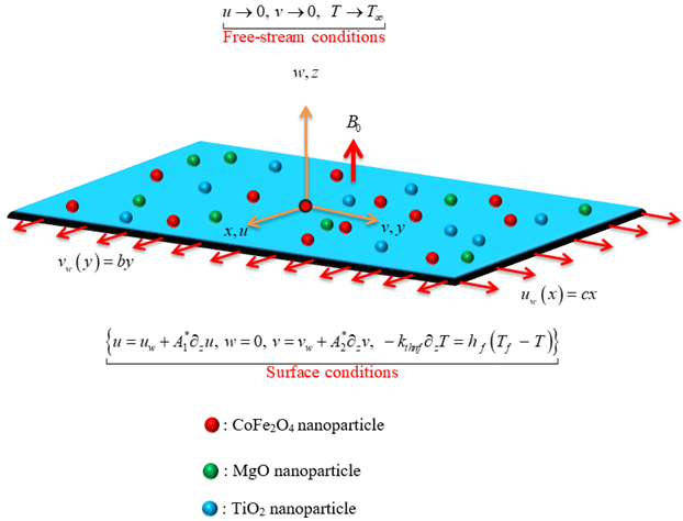
We examined ternary hybrid Carreau nanofluid flow on a porous bi-directional elongating sheet. The nanoparticles of TiO₂, CoFe₂O₄, and MgO were mixed with water to get a ternary hybrid nanofluid. The flow was influenced by slip conditions of velocities along the x- and y-axes. The impacts of thermal- and space-dependent heat sources, thermal radiation, viscous dissipation, and Joule heating were used in this study. Moreover, magnetic effects were used along the z-axis, which was normal to the flow direction. The major equations were solved using the homotopy analysis method (HAM) in dimensionless form. As an outcome of this study, we discovered that with progression in velocity slip factors along x- and y-axes, magnetic factor, porosity factor, and local Weissenberg number, there was a reduction in primary and secondary velocities. With an upsurge in the stretching ratio factor, there was a reduction in primary flow and augmentation in secondary flow. Thermal distribution was augmented with the surge in thermal Biot number, thermal-dependent heat source factor, magnetic factor, space-dependent heat source parameter, radiation factor, and Eckert numbers along primary and secondary directions. The skin friction coefficients have augmented with growth in magnetic factor, porosity factor, and velocity slip factors along the x- and y-axes. The Nusselt number escalated with a surge in radiation factor, space-dependent heat source factor, thermal-dependent heat source factor, and Eckert numbers along x- and y-axes. Our results were validated through comparative analysis by matching our results with established data. A fine agreement was noticed among all the results. Our findings benefit aerospace, biomedical, and electronics industries by improving thermal management in porous media. Magnetic and slip conditions aid in advanced manufacturing, while enhanced Nusselt numbers support efficient heat exchanger design.

References

[1]	S. U. S. Choi, J. A. Eastman, Enhancing thermal conductivity of fluids with nanoparticles, Argonne National Lab. (ANL), Argonne, IL (United States), 1995.
[2]	A. Ali, Z. Khan, M. Sun, T. Muhammad, K. A. M. Alharbi, Numerical investigation of heat and mass transfer in micropolar nanofluid flows over an inclined surface with stochastic numerical approach, Eur. Phys. J. Plus, 139 (2024), 1–25. https://doi.org/10.1140/epjp/s13360-024-05676-0 doi: 10.1140/epjp/s13360-024-05676-0
[3]	A. M. Galal, F. M. Alharbi, M. Arshad, M. M. Alam, T. Abdeljawad, Q. M. Al-Mdallal, Numerical investigation of heat and mass transfer in three-dimensional MHD nanoliquid flow with inclined magnetization, Sci. Rep., 14 (2024), 1207. https://doi.org/10.1038/s41598-024-51195-4 doi: 10.1038/s41598-024-51195-4
[4]	E. A. Algehyne, F. M. Alamrani, A. Khan, K. A. Khan, S. A. Lone, A. Saeed, A comparative analysis of the blood-based hybrid nanofluid flow containing Cu and CuO nanoparticles over an exponentially extending surface, Proc. I. Mech. Eng. E-J. Proc., 2024. https://doi.org/10.1177/09544089241235063
[5]	V. P. Kalbande, M. S. Choudhari, Y. N. Nandanwar, Hybrid nano-fluid for solar collector based thermal energy storage and heat transmission systems: A review, J. Energy Storage, 86 (2024), 111243. https://doi.org/10.1016/j.est.2024.111243 doi: 10.1016/j.est.2024.111243
[6]	A. Kazemian, A. Salari, T. Ma, H. Lu, Application of hybrid nanofluids in a novel combined photovoltaic/thermal and solar collector system, Sol. Energy, 239 (2022), 102–116. https://doi.org/10.1016/j.solener.2022.04.016 doi: 10.1016/j.solener.2022.04.016
[7]	K. Guedri, A. Khan, N. Sene, Z. Raizah, A. Saeed, A. M. Galal, Thermal flow for radiative ternary hybrid nanofluid over nonlinear stretching sheet subject to Darcy-Forchheimer phenomenon, Math. Probl. Eng., 2022 (2022). https://doi.org/10.1155/2022/3429439
[8]	Y. Mehmood, A. Alsinai, M. Bilal, S. Iqbal, A. U. K. Niazi, N. Faisal, Numerical investigation of entropy generation on micropolar trihybrid nanofluid flow with blood as base fluid in a channel, J. Math., 2024 (2024), 9583109. https://doi.org/10.1155/2024/9583109 doi: 10.1155/2024/9583109
[9]	S. Z. H. Shah, A. Ayub, S. Bhatti, U. Khan, A. Ishak, E. M. Sherif, et al., Aspects of inclined magnetohydrodynamics and heat transfer in a non‐Newtonian tri‐hybrid bio‐nanofluid flow past a wedge‐shaped artery utilizing artificial neural network scheme, ZAMM‐J. Appl. Math. Mech. Für Angew. Math. Und Mech., 104 (2024), e202400278. https://doi.org/10.1002/zamm.202400278 doi: 10.1002/zamm.202400278
[10]	M. I. I. Rabby, M. W. Uddin, N. M. S. Hassan, M. Al Nur, R. Uddin, S. Istiaque, et al., Recent progresses in tri-hybrid nanofluids: A comprehensive review on preparation, stability, thermo-hydraulic properties, and applications, J. Mol. Liq., 2024, 125257. https://doi.org/10.1016/j.molliq.2024.125257
[11]	M. D. Afifi, B. Jalili, A. Mirzaei, P. Jalili, D. Ganji, The effects of thermal radiation, thermal conductivity, and variable viscosity on ferrofluid in porous medium under magnetic field, World J. Eng., 22 (2025), 218–231. http://org. doi/10.1108/WJE-09-2023-0402 doi: 10.1108/WJE-09-2023-0402
[12]	S. Anwar, U. Ahmad, T. Sun, M. Ashraf, G. Rasool, Impact of solar radiation in the presence of temperature-dependent thermal conductivity of non-Newtonian Casson flow on natural convection heat transfer in plume generated due to the combined effects of heat source and aligned magnetic field, Numer. Heat Transf. Part A Appl., 2024, 1–18. https://doi.org/10.1080/10407782.2024.2367089
[13]	G. Sarfraz, S. U. Khan, D. L. C. Ching, I. Khan, A. Mir, Y. Khan, et al., Influence of solar thermal radiations and convective boundary on Al2O₃/H₂O transient model efficiency, J. Radiat. Res. Appl. Sci., 17 (2024), 101117. https://doi.org/10.1016/j.jrras.2024.101117 doi: 10.1016/j.jrras.2024.101117
[14]	M. Nayfeh, A. Nayfeh, A. Rezk, E. Bahceci, W. Alnaser, On silicon nanobubbles in space for scattering and interception of solar radiation to ease high-temperature induced climate change, AIP Adv., 14 (2024). https://doi.org/10.1063/5.0187880
[15]	S. Nasir, A. Berrouk, Z. Khan, Efficiency assessment of thermal radiation utilizing flow of advanced nanocomposites on riga plate, Appl. Therm. Eng., 242 (2024), 122531. https://doi.org/10.1016/j.applthermaleng.2024.122531 doi: 10.1016/j.applthermaleng.2024.122531
[16]	M. Sohail, K. Abodayeh, U. Nazir, Implementation of finite element scheme to study thermal and mass transportation in water-based nanofluid model under quadratic thermal radiation in a disk, Mech. Time-Depend. Mater., 28 (2024), 1049–1072. https://doi.org/10.1007/s11043-024-09736-x doi: 10.1007/s11043-024-09736-x
[17]	U. Farooq, A. Jan, M. Hussain, Impact of thermal radiations, heat generation/absorption and porosity on MHD nanofluid flow towards an inclined stretching surface: Non‐similar analysis, ZAMM‐J. Appl. Math. Mech. Für Angew. Math. Und Mech., 104 (2024), e202300306. https://doi.org/10.1002/zamm.202300306 doi: 10.1002/zamm.202300306
[18]	S. Bilal, M. B. Riaz, Thermofluidic transport of Williamson flow in stratified medium with radiative energy and heat source aspects by machine learning paradigm, Int. J. Thermofluids, 24 (2024), 100818. https://doi.org/10.1016/j.ijft.2024.100818 doi: 10.1016/j.ijft.2024.100818
[19]	B. Ali, S. Jubair, M. I. H. Siddiqui, Numerical simulation of 3D Darcy-Forchheimer hybrid nanofluid flow with heat source/sink and partial slip effect across a spinning disc, J. Porous Media, 27 (2024). https://doi.org/10.1615/JPorMedia.2024051759
[20]	P. Jalili, S. M. S. Mousavi, B. Jalili, P. Pasha, D. D. Ganji, Thermal evaluation of MHD Jeffrey fluid flow in the presence of a heat source and chemical reaction, Int. J. Mod. Phys. B, 38 (2024), 2450113. https://doi.org/10.1142/S0217979224501133 doi: 10.1142/S0217979224501133
[21]	K. Alqawasmi, K. A. M. Alharbi, U. Farooq, S. Noreen, M. Imran, A. Akgül, et al., Numerical approach toward ternary hybrid nanofluid flow with nonlinear heat source-sink and fourier heat flux model passing through a disk, Int. J. Thermofluids, 18 (2023), 100367. https://doi.org/10.1016/j.ijft.2023.100367 doi: 10.1016/j.ijft.2023.100367
[22]	J. K. Madhukesh, I. E. Sarris, V. K, B. C. Prasannakumara, A. Abdulrahman, Computational analysis of ternary nanofluid flow in a microchannel with nonuniform heat source/sink and waste discharge concentration, Numer. Heat Tr. A-Appl., 2023, 1–18. https://doi.org/10.1080/10407782.2023.2240509
[23]	G. Shankar, P. Deepalakshmi, E. P. Siva, D. Tripathi, O. A. Bég, Thermomagnetic peristaltic Casson flow in a microchannel containing a Darcy–Brinkman porous medium under the influence of oscillatory, thermal radiation, slip and heat source effects, Pramana, 99 (2025), 32. https://doi.org/10.1007/s12043-024-02869-1 doi: 10.1007/s12043-024-02869-1
[24]	M. V. Reddy, K. Vajravelu, P. Lakshminarayana, G. Sucharitha, Heat source and Joule heating effects on convective MHD stagnation point flow of Casson nanofluid through a porous medium with chemical reaction, Numer. Heat Tr. B-Fund., 85 (2024), 286–304. https://doi.org/10.1080/10407790.2023.2233694 doi: 10.1080/10407790.2023.2233694
[25]	M. Abbas, N. Khan, M. S. Hashmi, R. K. Alhefthi, S. Rezapour, M. Inc, Thermal Marangoni convection in two-phase quadratic convective flow of dusty MHD trihybrid nanofluid with non-linear heat source, Case Stud. Therm. Eng., 57 (2024), 104190. https://doi.org/10.1016/j.csite.2024.104190 doi: 10.1016/j.csite.2024.104190
[26]	K. Swain, S. M. Ibrahim, G. Dharmaiah, S. Noeiaghdam, Numerical study of nanoparticles aggregation on radiative 3D flow of maxwell fluid over a permeable stretching surface with thermal radiation and heat source/sink, Results Eng., 19 (2023), 101208. https://doi.org/10.1016/j.rineng.2023.101208 doi: 10.1016/j.rineng.2023.101208
[27]	T. Salahuddin, G. Fatima, M. Awais, M. Khan, B. Al Awan, Adaptation of nanofluids with magnetohydrodynamic Williamson fluid to enhance the thermal and solutal flow analysis with viscous dissipation: A numerical study, Results Eng., 21 (2024), 101798. https://doi.org/10.1016/j.rineng.2024.101798 doi: 10.1016/j.rineng.2024.101798
[28]	N. B. Khedher, Z. Ullah, Y. M. Mahrous, S. Dhahbi, S. Ahmad, H. Abu-Zinadah, et al., Viscous dissipation effect on amplitude and oscillating frequency of heat transfer and electromagnetic waves of magnetic driven fluid flow along the horizontal circular cylinder, Case Stud. Therm. Eng., 55 (2024), 104142. https://doi.org/10.1016/j.csite.2024.104142 doi: 10.1016/j.csite.2024.104142
[29]	A. Rehman, M. C. Khun, A. S. Alsubaie, M. Inc, Influence of Marangoni convection, viscous dissipation, and variable fluid viscosity of nanofluid flow on stretching surface analytical analysis, ZAMM‐J. Appl. Math. Mech. Für Angew. Math. Und Mech., 104 (2024), e202300413. https://doi.org/10.1002/zamm.202300413 doi: 10.1002/zamm.202300413
[30]	S. Akram, K. Saeed, M. Athar, A. Riaz, A. Razia, M. A. S. Al-Malki, Enhancing retention of biological fluid transport of magnetized thermal radiative pseudoplastic nanofluid with double diffusion convection, viscous dissipation and boundary slips, Part. Sci. Technol., 43 (2025), 1–14. https://doi.org/10.1080/02726351.2024.2412654 doi: 10.1080/02726351.2024.2412654
[31]	S. Li, S. Akbar, M. Sohail, U. Nazir, A. Singh, M. Alanazi, et al., Influence of buoyancy and viscous dissipation effects on 3D magneto hydrodynamic viscous hybrid nano fluid (MgO−TiO₂) under slip conditions, Case Stud. Therm. Eng., 49 (2023), 103281. https://doi.org/10.1016/j.csite.2023.103281 doi: 10.1016/j.csite.2023.103281
[32]	B. Alqahtani, E. R. El-Zahar, M. B. Riaz, L. F. Seddek, A. Ilyas, Z. Ullah, et al., Computational analysis of microgravity and viscous dissipation impact on periodical heat transfer of MHD fluid along porous radiative surface with thermal slip effects, Case Stud. Therm. Eng., 60 (2024), 104641. https://doi.org/10.1016/j.csite.2024.104641 doi: 10.1016/j.csite.2024.104641
[33]	N. Abid, J. Hasnain, Viscous dissipation effects on the axisymmetric flow of Casson rheological fluid in the core region of curved artery surrounded by Al₂O₃/γ-Al₂O₃ nanofluid, Int. J. Heat Fluid Flow., 107 (2024), 109349. https://doi.org/10.1016/j.ijheatfluidflow.2024.109349 doi: 10.1016/j.ijheatfluidflow.2024.109349
[34]	M. Irfan, I. Siddique, K. A. Gepreel, M. Nazeer, D. Abduvalieva, M. I. Khan, Investigation of heat transfer phenomenon in a complex wavy divergent channel under the effects of thermal radiation, joule heating and electroosmosis, Numer. Heat Tr. A-Appl., 2024, 1–20. https://doi.org/10.1080/10407782.2024.2386033
[35]	N. Elboughdiri, K. Javid, P. Lakshminarayana, A. Abbasi, Y. Benguerba, Effects of Joule heating and viscous dissipation on EMHD boundary layer rheology of viscoelastic fluid over an inclined plate, Case Stud. Therm. Eng., 60 (2024), 104602. https://doi.org/10.1016/j.csite.2024.104602 doi: 10.1016/j.csite.2024.104602
[36]	N. Hasan, S. Saha, Effects of internal heat production and Joule heating on MHD conjugate mixed convection and entropy production inside a thermally non-homogeneous cooling system, Ann. Nucl. Energy, 206 (2024), 110671. https://doi.org/10.1016/j.anucene.2024.110671 doi: 10.1016/j.anucene.2024.110671
[37]	E. Ghaderi, M. Bijarchi, S. K. Hannani, A. Nouri-Borujerdi, Evaluating Joule heating influence on heat transfer and entropy generation in MHD channel flow: A parametric study and ill-posed problem solution using PINNs, arXiv preprint, 2024. https://doi.org/10.48550/arXiv.2406.15810
[38]	A. Ullah, H. Yao, F. Ullah, W. Khan, H. Gul, F. A. Awwad, et al., Viscous dissipation and Joule heating effects on the unsteady micropolar fluid flow past a horizontal surface of revolution, Alex. Eng. J., 94 (2024), 159–171. https://doi.org/10.1016/j.aej.2024.03.032 doi: 10.1016/j.aej.2024.03.032
[39]	T. Abdeljawad, M. Sohail, D. R. Mostapha, Impacts of Hall current and Joule heating of Cattaneo-Christov on peristaltic stenosed artery of Reiner-Rivlin liquid through Darcy-Forchheimer feature, Ain Shams Eng. J., 15 (2024), 102679. https://doi.org/10.1016/j.asej.2024.102679 doi: 10.1016/j.asej.2024.102679
[40]	A. Tahiri, H. Ragueb, M. Moussaoui, K. Mansouri, D. Guerraiche, K. Guerraiche, Heat transfer and entropy generation in viscous-joule heating MHD microchannels flow under asymmetric heating, Int. J. Numer. Method. H., 34 (2024), 3953–3978. Available from: https://www.researchgate.net/publication/383332552.
[41]	H. Waqas, M. Imran, M. M. Bhatti, Bioconvection aspects in non-Newtonian three-dimensional Carreau nanofluid flow with Cattaneo–Christov model and activation energy, Eur. Phys. J. Spec. Top., 230 (2021), 1317–1330. https://doi.org/10.1140/epjs/s11734-021-00046-8 doi: 10.1140/epjs/s11734-021-00046-8
[42]	T. Hayat, A. Aziz, T. Muhammad, A. Alsaedi, Numerical simulation for three-dimensional flow of Carreau nanofluid over a nonlinear stretching surface with convective heat and mass conditions, J. Braz. Soc. Mech. Sci. Eng., 41 (2019), 1–11. https://doi.org/10.1007/S40430-018-1540-7 doi: 10.1007/S40430-018-1540-7
[43]	K. G. Kumar, G. K. Ramesh, B. J. Gireesha, R. S. R. Gorla, Characteristics of Joule heating and viscous dissipation on three-dimensional flow of Oldroyd B nanofluid with thermal radiation, Alex. Eng. J., 57 (2018), 2139–2149. https://doi.org/10.1016/j.aej.2017.06.006 doi: 10.1016/j.aej.2017.06.006
[44]	T. Muhammad, T. Hayat, S. A. Shehzad, A. Alsaedi, Viscous dissipation and Joule heating effects in MHD 3D flow with heat and mass fluxes, Results Phys., 8 (2018), 365–371. https://doi.org/10.1016/j.rinp.2017.12.047 doi: 10.1016/j.rinp.2017.12.047
[45]	P. Priyadharshini, M. V. Archana, N. A. Shah, M. H. Alshehri, Ternary hybrid nanofluid flow emerging on a symmetrically stretching sheet optimization with machine learning prediction scheme, Symmetry, 15 (2023), 1225. https://doi.org/10.3390/sym15061225 doi: 10.3390/sym15061225
[46]	N. Acharya, S. Maity, P. K. Kundu, Framing the hydrothermal features of magnetized TiO₂–CoFe₂O₄ water-based steady hybrid nanofluid flow over a radiative revolving disk, Multidiscip. Model. Ma., 16 (2020), 765–790. https://doi.org/10.1108/MMMS-08-2019-0151 doi: 10.1108/MMMS-08-2019-0151
[47]	K. A. M. Alharbi, A. E. S. Ahmed, M. O. Sidi, N. A. Ahammad, A. Mohamed, M. A. El-Shorbagy, et al., Computational valuation of Darcy ternary-hybrid nanofluid flow across an extending cylinder with induction effects, Micromachines, 13 (2022), 588. https://doi.org/10.3390/mi13040588 doi: 10.3390/mi13040588
[48]	F. Wang, U. Nazir, M. Sohail, E. R. El-Zahar, C. Park, P. Thounthong, A Galerkin strategy for tri-hybridized mixture in ethylene glycol comprising variable diffusion and thermal conductivity using non-Fourier's theory, Nanotechnol. Rev., 11 (2022), 834–845. https://doi.org/10.1515/ntrev-2022-0050 doi: 10.1515/ntrev-2022-0050
[49]	B. Unyong, R. Vadivel, M. Govindaraju, R. Anbuvithya, N. Gunasekaran, Entropy analysis for ethylene glycol hybrid nanofluid flow with elastic deformation, radiation, non-uniform heat generation/absorption, and inclined Lorentz force effects, Case Stud. Therm. Eng., 30 (2022), 101639. https://doi.org/10.1016/j.csite.2021.101639 doi: 10.1016/j.csite.2021.101639
[50]	T. S. Kumar, Hybrid nanofluid slip flow and heat transfer over a stretching surface, Part. Differ. Equ. Appl. Math., 4 (2021), 100070. https://doi.org/10.1016/j.padiff.2021.100070 doi: 10.1016/j.padiff.2021.100070
[51]	F. Wang, E. O. Fatunmbi, A. T. Adeosun, S. O. Salawu, I. L. Animasaun, I. E. Sarris, Comparative analysis between copper ethylene-glycol and copper-iron oxide ethylene-glycol nanoparticles both experiencing Coriolis force, velocity and temperature jump, Case Stud. Therm. Eng., 47 (2023), 103028. https://doi.org/10.1016/j.csite.2023.103028 doi: 10.1016/j.csite.2023.103028
[52]	T. A. Yusuf, F. Mabood, W. A. Khan, J. A. Gbadeyan, Irreversibility analysis of Cu-TiO₂-H₂O hybrid-nanofluid impinging on a 3-D stretching sheet in a porous medium with nonlinear radiation: Darcy-Forchhiemer's model, Alex. Eng. J., 59 (2020), 5247–5261. https://doi.org/10.1016/j.aej.2020.09.053 doi: 10.1016/j.aej.2020.09.053
[53]	F. Mabood, K. Das, Melting heat transfer on hydromagnetic flow of a nanofluid over a stretching sheet with radiation and second-order slip, Eur. Phys. J. Plus., 131 (2016), 1–12. https://doi.org/10.1140/epjp/i2016-16003-1 doi: 10.1140/epjp/i2016-16003-1
[54]	L. Xu, E. W. M. Lee, Variational iteration method for the magnetohydrodynamic flow over a nonlinear stretching sheet, Abstr. Appl. Anal., 2013, 573782. https://doi.org/10.1155/2013/573782

Reader Comments

Your name:*

Email:*
© 2025 the Author(s), licensee AIMS Press. This is an open access article distributed under the terms of the Creative Commons Attribution License (http://creativecommons.org/licenses/by/4.0)