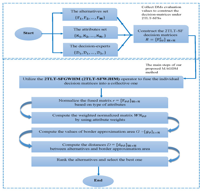
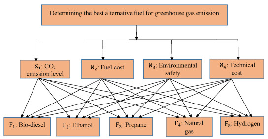
In recent years, fossil fuel resources have become increasingly rare and caused a variety of problems, with a global impact on economy, society and environment. To tackle this challenge, we must promote the development and diffusion of alternative fuel technologies. The use of cleaner fuels can reduce not only economic cost but also the emission of gaseous pollutants that deplete the ozone layer and accelerate global warming. To select an optimal alternative fuel, different fuzzy decision analysis methodologies can be utilized. In comparison to other extensions of fuzzy sets, the $ T $-spherical fuzzy set is an emerging tool to cope with uncertainty by quantifying acceptance, abstention and rejection jointly. It provides a general framework to unify various fuzzy models including fuzzy sets, picture fuzzy sets, spherical fuzzy sets, intuitionistic fuzzy sets, Pythagorean fuzzy sets and generalized orthopair fuzzy sets. Meanwhile, decision makers prefer to employ linguistic terms when expressing qualitative evaluation in real-life applications. In view of these facts, we develop an extended multi-attributive border approximation area comparison (MABAC) method for solving multiple attribute group decision-making problems in this study. Firstly, the combination of $ T $-spherical fuzzy sets with 2-tuple linguistic representation is presented, which provides a general framework for expressing and computing qualitative evaluation. Secondly, we put forward four kinds of 2-tuple linguistic $ T $-spherical fuzzy aggregation operators by considering the Heronian mean operator. We investigate some fundamental properties of the proposed 2-tuple linguistic $ T $-spherical fuzzy aggregation operators. Lastly, an extended MABAC method based on the 2-tuple linguistic $ T $-spherical fuzzy generalized weighted Heronian mean and the 2-tuple linguistic $ T $-spherical fuzzy weighted geometric Heronian mean operators is developed. For illustration, a case study on fuel technology selection with 2-tuple linguistic $ T $-spherical fuzzy information is also conducted. Moreover, we show the validity and feasibility of our approach by comparing it with several existing approaches.
Citation: Muhammad Akram, Sumera Naz, Feng Feng, Ghada Ali, Aqsa Shafiq. Extended MABAC method based on 2-tuple linguistic $ T $-spherical fuzzy sets and Heronian mean operators: An application to alternative fuel selection[J]. AIMS Mathematics, 2023, 8(5): 10619-10653. doi: 10.3934/math.2023539
In recent years, fossil fuel resources have become increasingly rare and caused a variety of problems, with a global impact on economy, society and environment. To tackle this challenge, we must promote the development and diffusion of alternative fuel technologies. The use of cleaner fuels can reduce not only economic cost but also the emission of gaseous pollutants that deplete the ozone layer and accelerate global warming. To select an optimal alternative fuel, different fuzzy decision analysis methodologies can be utilized. In comparison to other extensions of fuzzy sets, the $ T $-spherical fuzzy set is an emerging tool to cope with uncertainty by quantifying acceptance, abstention and rejection jointly. It provides a general framework to unify various fuzzy models including fuzzy sets, picture fuzzy sets, spherical fuzzy sets, intuitionistic fuzzy sets, Pythagorean fuzzy sets and generalized orthopair fuzzy sets. Meanwhile, decision makers prefer to employ linguistic terms when expressing qualitative evaluation in real-life applications. In view of these facts, we develop an extended multi-attributive border approximation area comparison (MABAC) method for solving multiple attribute group decision-making problems in this study. Firstly, the combination of $ T $-spherical fuzzy sets with 2-tuple linguistic representation is presented, which provides a general framework for expressing and computing qualitative evaluation. Secondly, we put forward four kinds of 2-tuple linguistic $ T $-spherical fuzzy aggregation operators by considering the Heronian mean operator. We investigate some fundamental properties of the proposed 2-tuple linguistic $ T $-spherical fuzzy aggregation operators. Lastly, an extended MABAC method based on the 2-tuple linguistic $ T $-spherical fuzzy generalized weighted Heronian mean and the 2-tuple linguistic $ T $-spherical fuzzy weighted geometric Heronian mean operators is developed. For illustration, a case study on fuel technology selection with 2-tuple linguistic $ T $-spherical fuzzy information is also conducted. Moreover, we show the validity and feasibility of our approach by comparing it with several existing approaches.

| [1] |
M. Agarwal, K. K. Biswas, M. Hanmandlu, Generalized intuitionistic fuzzy soft sets with applications in decision-making, Appl. Soft Comput., 13 (2013), 3552â€"3566. https://doi.org/10.1016/j.asoc.2013.03.015 doi: 10.1016/j.asoc.2013.03.015

|
| [2] |
M. Akram, S. Naz, F. Feng, A. Shafiq, Assessment of hydropower plants in Pakistan: Muirhead mean-based 2-tuple linguistic $T$-spherical fuzzy model combining SWARA with COPRAS, Arab. J. Sci. Eng., 2022, 1â€"30. https://doi.org/10.1007/s13369-022-07081-0 doi: 10.1007/s13369-022-07081-0
|
| [3] |
M. Akram, S. Naz, G. Santos-Garcia, M. R. Saeed, Extended CODAS method for MAGDM with 2-tuple linguistic $T$-spherical fuzzy sets, AIMS Math., 8 (2023), 3428â€"3468. https://doi.org/10.3934/math.2023176 doi: 10.3934/math.2023176
|
| [4] |
M. Akram, C. Kahraman, K. Zahid, Group decision-making based on complex spherical fuzzy VIKOR approach, Knowl.-Based Syst., 216 (2021), 106â€"793. https://doi.org/10.1016/j.knosys.2021.106793 doi: 10.1016/j.knosys.2021.106793
|
| [5] |
M. Akram, X. Peng, A. Sattar, A new decision-making model using complex intuitionistic fuzzy Hamacher aggregation operators, Soft Comput., 25 (2021), 7059â€"7086. https://doi.org/10.1007/s00500-021-05658-9 doi: 10.1007/s00500-021-05658-9
|
| [6] |
M. Akram, C. Kahraman, K. Zahid, Extension of TOPSIS model to the decision-making under complex spherical fuzzy information, Soft Comput., 25 (2021), 10771â€"10795. https://doi.org/10.1007/s00500-021-05945-5 doi: 10.1007/s00500-021-05945-5
|
| [7] |
M. Akram, A. Martino, Multi-attribute group decision making based on $T$-spherical fuzzy soft rough average aggregation operators, Granular Comput., 8 (2023), 171â€"207. https://doi.org/10.1007/s41066-022-00319-0 doi: 10.1007/s41066-022-00319-0
|
| [8] | M. Akram, R. Bibi, M. Deveci, An outranking approach with 2-tuple linguistic Fermatean fuzzy sets for multi-attribute group decision-making, Eng. Appl. Artif. Intell., 121 (2023). |
| [9] |
M. Akram, N. Ramzan, M. Deveci, Linguistic Pythagorean fuzzy CRITIC-EDAS method for multiple-attribute group decision analysis, Eng. Appl. Artif. Intell., 119 (2023), 105777. https://doi.org/10.1016/j.engappai.2022.105777 doi: 10.1016/j.engappai.2022.105777
|
| [10] |
M. Akram, A. Khan, A. Luqman, T. Senapati, D. Pamucar, An extended MARCOS method for MCGDM under 2-tuple linguistic q-rung picture fuzzy environment, Eng. Appl. Artif. Intell., 120 (2023), 105892. https://doi.org/10.1016/j.engappai.2023.105892 doi: 10.1016/j.engappai.2023.105892
|
| [11] |
M. Akram, Z. Niaz, F. Feng, Extended CODAS method for multi-attribute group decision-making based on 2-tuple linguistic Fermatean fuzzy Hamacher aggregation operators, Granul. Comput., 2022. https://doi.org/10.1007/s41066-022-00332-3 doi: 10.1007/s41066-022-00332-3
|
| [12] |
K. T. Atanassov, Intuitionistic fuzzy sets, Fuzzy Set. Syst., 20 (1986), 87â€"96. https://doi.org/10.1016/S0165-0114(86)80034-3 doi: 10.1016/S0165-0114(86)80034-3
|
| [13] | A. Azapagic, Sustainable production and consumption: A decision-support framework integrating environmental, economic and social sustainability, Comput. Aided Chem. Eng., 37 (2015), 131â€"136. |
| [14] | G. Beliakov, A. Pradera, T. Calvo, Aggregation functions: A guide for practitioners, Springer, Berlin, Heidelberg, 221 (2007), 361. |
| [15] | B. C. Cuong, V. Kreinovich, Picture fuzzy sets, J. Comput. Sci. Cyb., 30 (2014), 409â€"420. |
| [16] |
X. Deng, J. Wang, G. Wei, Some 2-tuple linguistic Pythagorean Heronian mean operators and their application to multiple attribute decision-making, J. Exp. Theor. Artif. Intell., 31 (2019), 555â€"574. https://doi.org/10.1080/0952813X.2019.1579258 doi: 10.1080/0952813X.2019.1579258
|
| [17] |
F. Feng, H. Fujita, M. I. Ali, R. R. Yager, X. Liu, Another view on generalized intuitionistic fuzzy soft sets and related multiattribute decision making methods, IEEE T. Fuzzy Syst., 27 (2019), 474â€"488. https://doi.org/10.1109/TFUZZ.2018.2860967 doi: 10.1109/TFUZZ.2018.2860967
|
| [18] |
F. Feng, Z. Xu, H. Fujita, M. Liang, Enhancing PROMETHEE method with intuitionistic fuzzy soft sets, Int. J. Intell. Syst., 35 (2020), 1071â€"1104. https://doi.org/10.1002/int.22235 doi: 10.1002/int.22235
|
| [19] |
Y. Fu, R. Cai, B. Yu, Group decision-making method with directed graph under linguistic environment, Int. J. Mach. Learn. Cyb., 13 (2022), 3329â€"3340. https://doi.org/10.1007/s13042-022-01597-5 doi: 10.1007/s13042-022-01597-5
|
| [20] |
H. Garg, K. Ullah, T. Mahmood, N. Hassan, N. Jan, $T$-spherical fuzzy power aggregation operators and their applications in multi-attribute decision making, J. Amb. Intell. Hum. Comp., 12 (2021), 9067â€"9080. https://doi.org/10.1007/s12652-020-02600-z doi: 10.1007/s12652-020-02600-z
|
| [21] |
F. K. Gündogdu, C. Kahraman, Spherical fuzzy sets and spherical fuzzy TOPSIS method, J. Intell. Fuzzy Syst., 36 (2019), 337â€"352. https://doi.org/10.3233/JIFS-181401 doi: 10.3233/JIFS-181401
|
| [22] |
A. Guleria, R. K. Bajaj, $T$-spherical fuzzy soft sets and its aggregation operators with application in decision making, Sci. Iran., 28 (2021), 1014â€"1029. https://doi.org/10.24200/sci.2019.53027.3018 doi: 10.24200/sci.2019.53027.3018
|
| [23] |
L. Gigovic, D. Pamučar, D. Bozanic, S. Ljubojevic, Application of the GIS-DANP-MABAC multi-criteria model for selecting the location of wind farms: A case study of vojvodina, Serbia, Renew. Energ., 103 (2017), 501â€"521. https://doi.org/10.1016/j.renene.2016.11.057 doi: 10.1016/j.renene.2016.11.057
|
| [24] |
Y. He, X. Wang, J. Z. Huang, Recent advances in multiple criteria decision making techniques, Int. J. Mach. Learn. Cyb., 139 (2022), 561â€"564. https://doi.org/10.1007/s13042-015-0490-y doi: 10.1007/s13042-015-0490-y
|
| [25] |
F. Herrera, L. Martinez, An approach for combining linguistic and numerical information based on the 2-tuple fuzzy linguistic representation model in decision-making, Int. J. Uncertain. Fuzz. Knowl.-Based Syst., 8 (2000), 539â€"562. https://doi.org/10.1142/S0218488500000381 doi: 10.1142/S0218488500000381
|
| [26] |
S. Jiang, W. He, F. Qin, Q. Cheng, Multiple attribute group decision-making based on power Heronian aggregation operators under interval-valued dual hesitant fuzzy environment, Math. Probl. Eng., 2020 (2020), 1â€"19. https://doi.org/10.1155/2020/2080413 doi: 10.1155/2020/2080413
|
| [27] | C. Kahraman, F. K. Gündogdu, S. C. Onar, B. Ötaysi, Hospital location selection using spherical fuzzy TOPSIS, In 2019 Conference of the International Fuzzy Systems Association and the European Society for Fuzzy Logic and Technology (EUSFLAT 2019), Atlantis Press, 2019. https://dx.doi.org/10.2991/eusflat-19.2019.12 |
| [28] |
M. K. Ghorabaee, E. K. Zavadskas, L. Olfat, Z. Turskis, Multi-criteria inventory classification using a new method of evaluation based on distance from average solution (EDAS), Informatica, 26 (2015), 435â€"451. https://doi.org/10.15388/Informatica.2015.57 doi: 10.15388/Informatica.2015.57
|
| [29] | M. Keshavarz Ghorabaee, E. K. Zavadskas, Z. Turskis, J. Antucheviciene, A new combinative distance-based assessment (CODAS) method for multi-criteria decision-making, Econ. Comput. Econ. Cyb., 50 (2016), 25â€"44. |
| [30] |
D. Liang, Z. Xu, D. Liu, Y. Wu, Method for three-way decisions using ideal TOPSIS solutions at Pythagorean fuzzy information, Inform. Sci., 435 (2018), 282â€"295. https://doi.org/10.1016/j.ins.2018.01.015 doi: 10.1016/j.ins.2018.01.015
|
| [31] | W. F. Liu, J. Chin, Linguistic Heronian mean operators and applications in decision making, Manag. Sci., 25 (2017), 174â€"183. |
| [32] |
P. Liu, S. Naz, M. Akram, M. Muzammal, Group decision-making analysis based on linguistic $q$-rung orthopair fuzzy generalized point weighted aggregation operators, Int. J. Mach. Learn. Cyb., 13 (2022), 883â€"906. https://doi.org/10.1007/s13042-021-01425-2 doi: 10.1007/s13042-021-01425-2
|
| [33] |
P. Liu, B. Zhu, P. Wang, M. Shen, An approach based on linguistic spherical fuzzy sets for public evaluation of shared bicycles in China, Eng. Appl. Artif. Intel., 87 (2020), 103â€"295. https://doi.org/10.1016/j.engappai.2019.103295 doi: 10.1016/j.engappai.2019.103295
|
| [34] |
P. Liu, K. Zhang, P. Wang, F. Wang, A clustering-and maximum consensus-based model for social network large-scale group decision making with linguistic distribution, Inform. Sci., 602 (2022), 269â€"297. https://doi.org/10.1016/j.ins.2022.04.038 doi: 10.1016/j.ins.2022.04.038
|
| [35] |
Z. Liu, W. Wang, D. Wang, A modified ELECTRE â…¡ method with double attitude parameters based on linguistic Z-number and its application for third-party reverse logistics provider selection, Appl. Intell., 52 (2022), 14964â€"14987. https://doi.org/10.1007/s10489-022-03315-8 doi: 10.1007/s10489-022-03315-8
|
| [36] |
P. Liu, Y. Wu, Y. Li, Probabilistic hesitant fuzzy taxonomy method based on best-worst-method (BWM) and indifference threshold-based attribute ratio analysis (ITARA) for multi-attributes decision-making, Int. J. Fuzzy Syst., 24 (2022), 1301â€"1317. https://doi.org/10.1007/s40815-021-01206-7 doi: 10.1007/s40815-021-01206-7
|
| [37] |
P. Liu, Y. Li, X. Zhang, W. Pedrycz, A multiattribute group decision-making method with probabilistic linguistic information based on an adaptive consensus reaching model and evidential reasoning, IEEE T. Cyb., 53 (2022), 1905â€"1919. https://doi.org/10.1109/TCYB.2022.3165030 doi: 10.1109/TCYB.2022.3165030
|
| [38] | P. K. Maji, R. Biswas, A. R. Roy, Intuitionistic fuzzy soft sets, J. Fuzzy Math., 9 (2001), 677â€"692. |
| [39] |
T. Mahmood, K. Ullah, Q. Khan, N. Jan, An approach toward decision-making and medical diagnosis problems using the concept of spherical fuzzy sets, Neural Compu. Appl., 31 (2019), 7041â€"7053. https://doi.org/10.1007/s00521-018-3521-2 doi: 10.1007/s00521-018-3521-2
|
| [40] |
M. Munir, H. Kalsoom, K. Ullah, T. Mahmood, Y. M. Chu, $T$-spherical fuzzy einstein hybrid aggregation operators and their applications in multi-attribute decision making problems, Symmetry, 12 (2020), 365. https://doi.org/10.3390/sym12030365 doi: 10.3390/sym12030365
|
| [41] |
J. Mo, H. L. Huang, Archimedean geometric Heronian mean aggregation operators based on dual hesitant fuzzy set and their application to multiple attribute decision making, Soft Comput., 24 (2020), 1â€"13. https://doi.org/10.1007/s00500-020-04819-6 doi: 10.1007/s00500-020-04819-6
|
| [42] |
A. R. Mishra, A. Chandel, D. Motwani, Extended MABAC method based on divergence measures for multi-criteria assessment of programming language with interval-valued intuitionistic fuzzy sets, Granular Comput., 5 (2020), 97â€"117. https://doi.org/10.1007/s41066-018-0130-5 doi: 10.1007/s41066-018-0130-5
|
| [43] |
S. Narayanamoorthy, L. Ramya, S. Kalaiselvan, J. V. Kureethara, D. Kang, Use of DEMATEL and COPRAS method to select best alternative fuel for control of impact of greenhouse gas emissions, Socio-Econ. Plan. Sci., 76 (2021), 100â€"996. https://doi.org/10.1016/j.seps.2020.100996 doi: 10.1016/j.seps.2020.100996
|
| [44] |
S. Naz, M. Akram, G. Muhiuddin, A. Shafiq, Modified EDAS method for MAGDM based on MSM operators with 2-tuple linguistic $T$-spherical fuzzy sets, Math. Probl. Eng., 2022 (2022). https://doi.org/10.1155/2022/5075998 doi: 10.1155/2022/5075998
|
| [45] |
S. Naz, M. Akram, M. M. A. Al-Shamiri, M. R. Saeed, Evaluation of network security service provider using 2-tuple linguistic complex $q$-rung orthopair fuzzy COPRAS method, Complexity, 2022 (2022). https://doi.org/10.1155/2022/4523287 doi: 10.1155/2022/4523287
|
| [46] |
D. Pamučar, G. Ćirović, The selection of transport and handling resources in logistics centers using Multi-Attributive Border Approximation Area Comparison (MABAC), Expert Syst. Appl., 42 (2015), 3016â€"3028. https://doi.org/10.1016/j.eswa.2014.11.057 doi: 10.1016/j.eswa.2014.11.057
|
| [47] |
D. Pamučar, I. Petrović, Ćirović, Modification of the Best Worst and MABAC methods: A novel approach based on interval-valued fuzzy-rough numbers, Expert Syst. Appl., 91 (2018), 89â€"106. https://doi.org/10.1016/j.eswa.2017.08.042 doi: 10.1016/j.eswa.2017.08.042
|
| [48] |
X. Peng, Y. Yang, Pythagorean fuzzy choquet integral based MABAC method for multiple attribute group decision making, Int. J. Intell. Syst., 31 (2016), 989â€"1020. https://doi.org/10.1002/int.21814 doi: 10.1002/int.21814
|
| [49] |
S. G. Quek, G. Selvachandran, M. Munir, T. Mahmood, K. Ullah, L. H. Son, et al., Multi-attribute multi-perception decision-making based on generalized $T$-spherical fuzzy weighted aggregation operators on neutrosophic sets, Mathematics, 7 (2019), 780. https://doi.org/10.3390/math7090780 doi: 10.3390/math7090780
|
| [50] |
P. Rani, A. R. Mishra, Multi-criteria weighted aggregated sum product assessment framework for fuel technology selection using q-rung orthopair fuzzy sets, Sustain. Prod. Consump., 24 (2020), 90â€"104. https://doi.org/10.1016/j.spc.2020.06.015 doi: 10.1016/j.spc.2020.06.015
|
| [51] |
R. Sun, J. Hu, J. Zhou, X. Chen, A hesitant fuzzy linguistic projection-based MABAC method for patients' prioritization, Int. J. Fuzzy Syst., 20 (2018), 2144â€"2160. https://doi.org/10.1007/s40815-017-0345-7 doi: 10.1007/s40815-017-0345-7
|
| [52] |
K. Ullah, H. Garg, T. Mahmood, N. Jan, Z. Ali, Correlation coefficients for $T$-spherical fuzzy sets and their applications in clustering and multi-attribute decision making, Soft Comput., 24 (2020), 1647â€"1659. https://doi.org/10.1007/s00500-019-03993-6 doi: 10.1007/s00500-019-03993-6
|
| [53] |
K. Ullah, T. Mahmood, H. Garg, Evaluation of the performance of search and rescue robots using $T$-spherical fuzzy Hamacher aggregation operators, Int. J. Fuzzy Syst., 22 (2020), 570â€"582. https://doi.org/10.1007/s40815-020-00803-2 doi: 10.1007/s40815-020-00803-2
|
| [54] |
Y. X. Xue, J. X. You, X. D. Lai, H. C. Liu, An interval-valued intuitionistic fuzzy MABAC approach for material selection with incomplete weight information, Appl. Soft Comput., 38 (2016), 703â€"713. https://doi.org/10.1016/j.asoc.2015.10.010 doi: 10.1016/j.asoc.2015.10.010
|
| [55] |
M. Xue, P. Cao, B. Hou, Data-driven decision-making with weights and reliabilities for diagnosis of thyroid cancer, Int. J. Mach. Learn. Cyb., 13 (2022), 2257â€"2271. https://doi.org/10.1007/s13042-022-01521-x doi: 10.1007/s13042-022-01521-x
|
| [56] |
L. Yang, B. Li, Multiple-valued picture fuzzy linguistic set based on generalized Heronian mean operators and their applications in multiple attribute decision making, IEEE Access, 8 (2020), 86272â€"86295. https://doi.org/10.1109/ACCESS.2020.2992434 doi: 10.1109/ACCESS.2020.2992434
|
| [57] |
S. M. Yu, H. Zhou, X. H. Chen, J. Q. Wang, A multi-criteria decision-making method based on Heronian mean operators under a linguistic hesitant fuzzy environment, Asia-Pac. J. Oper. Res., 32 (2015), 1550035. https://doi.org/10.1142/S0217595915500359 doi: 10.1142/S0217595915500359
|
| [58] |
D. J. Yu, Intuitionistic fuzzy geometric Heronian mean aggregation operators, Appl. Soft Comput., 13 (2012), 1235â€"1246. https://doi.org/10.1016/j.asoc.2012.09.021 doi: 10.1016/j.asoc.2012.09.021
|
| [59] |
R. R. Yager, Pythagorean membership grades in multi-criteria decision-making, IEEE T. Fuzzy Syst., 22 (2014), 958â€"965. https://doi.org/10.1109/TFUZZ.2013.2278989 doi: 10.1109/TFUZZ.2013.2278989
|
| [60] |
R. R. Yager, Generalized orthopair fuzzy sets, IEEE T. Fuzzy Syst., 25 (2017), 1222â€"1230. https://doi.org/10.1109/TFUZZ.2016.2604005 doi: 10.1109/TFUZZ.2016.2604005
|
| [61] |
L. A. Zadeh, Fuzzy sets, Inform. Control, 8 (1965), 338â€"353. https://doi.org/10.1016/S0019-9958(65)90241-X doi: 10.1016/S0019-9958(65)90241-X
|
| [62] |
L. A. Zadeh, The concept of a linguistic variable and its application to approximate reasoning part â…, Inform. Sci., 8 (1975), 199â€"249. https://doi.org/10.1016/0020-0255(75)90036-5 doi: 10.1016/0020-0255(75)90036-5
|
| [63] |
L. Zhang, P. Zhu, Generalized fuzzy variable precision rough sets based on bisimulations and the corresponding decision-making, Int. J. Mach. Learn. Cyb., 13 (2022), 2313â€"2344. https://doi.org/10.1007/s13042-022-01527-5 doi: 10.1007/s13042-022-01527-5
|
| [64] |
M. Zhao, G. Wei, C. Wei, J. Wu, Improved TODIM method for intuitionistic fuzzy MAGDM based on cumulative prospect theory and its application on stock investment selection, Int. J. Mach. Learn. Cyb., 12 (2021), 891â€"901. https://doi.org/10.1007/s13042-020-01208-1 doi: 10.1007/s13042-020-01208-1
|
Figures(10) / Tables(18)

Muhammad Akram, Sumera Naz, Feng Feng, Ghada Ali, Aqsa Shafiq. Extended MABAC method based on 2-tuple linguistic $ T $-spherical fuzzy sets and Heronian mean operators: An application to alternative fuel selection[J]. AIMS Mathematics, 2023, 8(5): 10619-10653. doi: 10.3934/math.2023539


 DownLoad: