Fractional Timoshenko beam with a viscoelastically damped rotational component

Banan Al-Homidan; Nasser-eddine Tatar; Banan Al-Homidan; Nasser-eddine Tatar

doi:10.3934/math.20231256

AIMS Mathematics

2023, Volume 8, Issue 10: 24632-24662. doi: 10.3934/math.20231256

Previous Article Next Article

Research article

Fractional Timoshenko beam with a viscoelastically damped rotational component

Banan Al-Homidan ¹,
Nasser-eddine Tatar ^{2
,
,}

1.
Imam Abdulrahman bin Faisal University, Department of Mathematics, College of Sciences, P. O. Box 1982, Dammam, Saudi Arabia
2.
King Fahd University of Petroleum and Minerals, Department of Mathematics, Interdisciplinary Research Center for Intelligent Manufacturing and Robotics, Dhahran 31261, Saudi Arabia

Received: 13 April 2023 Revised: 24 June 2023 Accepted: 02 July 2023 Published: 21 August 2023
MSC : 26A33, 35B35, 35B40, 35L20

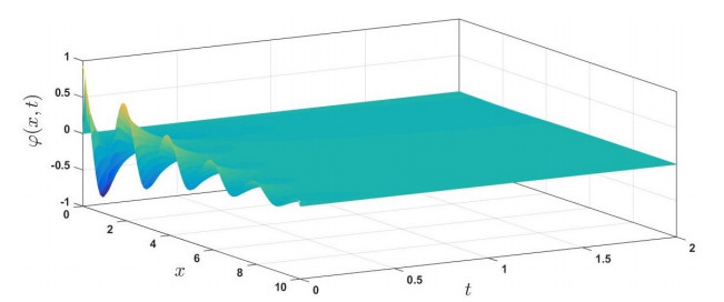
This paper is concerned with a fractional Timoshenko system of order between one and two. We address the question of well-posedness in an appropriate space when the rotational component is viscoelastic or subject to a viscoelastic controller. To this end we use the notion of alpha-resolvent. Moreover, we prove that the memory term alone may stabilize the system in a Mittag-Leffler fashion. The system is Lyapunov stable or uniformly stable in the case of different speeds of propagation.

Keywords:

Caputo fractional derivative,
Riemann-Liouville fractional derivative,
Mittag-Leffler stability,
Lyapunov stability,
multiplier technique

Citation: Banan Al-Homidan, Nasser-eddine Tatar. Fractional Timoshenko beam with a viscoelastically damped rotational component[J]. AIMS Mathematics, 2023, 8(10): 24632-24662. doi: 10.3934/math.20231256

Related Papers:

[1]	Mansour Shrahili, Mohamed Kayid . Uncertainty quantification based on residual Tsallis entropy of order statistics. AIMS Mathematics, 2024, 9(7): 18712-18731. doi: 10.3934/math.2024910
[2]	Ramy Abdelhamid Aldallal, Haroon M. Barakat, Mohamed Said Mohamed . Exploring weighted Tsallis extropy: Insights and applications to human health. AIMS Mathematics, 2025, 10(2): 2191-2222. doi: 10.3934/math.2025102
[3]	H. M. Barakat, M. A. Alawady, I. A. Husseiny, M. Nagy, A. H. Mansi, M. O. Mohamed . Bivariate Epanechnikov-exponential distribution: statistical properties, reliability measures, and applications to computer science data. AIMS Mathematics, 2024, 9(11): 32299-32327. doi: 10.3934/math.20241550
[4]	Mohamed Said Mohamed, Najwan Alsadat, Oluwafemi Samson Balogun . Continuous Tsallis and Renyi extropy with pharmaceutical market application. AIMS Mathematics, 2023, 8(10): 24176-24195. doi: 10.3934/math.20231233
[5]	Mohamed Said Mohamed, Haroon M. Barakat, Aned Al Mutairi, Manahil SidAhmed Mustafa . Further properties of Tsallis extropy and some of its related measures. AIMS Mathematics, 2023, 8(12): 28219-28245. doi: 10.3934/math.20231445
[6]	Refah Alotaibi, Mazen Nassar, Zareen A. Khan, Wejdan Ali Alajlan, Ahmed Elshahhat . Entropy evaluation in inverse Weibull unified hybrid censored data with application to mechanical components and head-neck cancer patients. AIMS Mathematics, 2025, 10(1): 1085-1115. doi: 10.3934/math.2025052
[7]	Alaa M. Abd El-Latif, Hanan H. Sakr, Mohamed Said Mohamed . Fractional generalized cumulative residual entropy: properties, testing uniformity, and applications to Euro Area daily smoker data. AIMS Mathematics, 2024, 9(7): 18064-18082. doi: 10.3934/math.2024881
[8]	M. Nagy, H. M. Barakat, M. A. Alawady, I. A. Husseiny, A. F. Alrasheedi, T. S. Taher, A. H. Mansi, M. O. Mohamed . Inference and other aspects for $q-$ Weibull distribution via generalized order statistics with applications to medical datasets. AIMS Mathematics, 2024, 9(4): 8311-8338. doi: 10.3934/math.2024404
[9]	Areej M. AL-Zaydi . On concomitants of generalized order statistics arising from bivariate generalized Weibull distribution and its application in estimation. AIMS Mathematics, 2024, 9(8): 22002-22021. doi: 10.3934/math.20241069
[10]	G. M. Mansour, M. A. Abd Elgawad, A. S. Al-Moisheer, H. M. Barakat, M. A. Alawady, I. A. Husseiny, M. O. Mohamed . Bivariate Epanechnikov-Weibull distribution based on Sarmanov copula: properties, simulation, and uncertainty measures with applications. AIMS Mathematics, 2025, 10(5): 12689-12725. doi: 10.3934/math.2025572

Abstract

1. Introduction

Chaos theory is the branch of mathematics that deals with complex behavior emerging in dynamical systems ^[1]. Chaotic systems possess special features such as extreme sensitivity to initial conditions, random-like unpredictable behavior and ergodicity. Improving these characteristics enhance applications in almost every field of science and engineering, such as: Biology ^[2], astrophysics ^[3], mechanics ^[4], economics ^[5], secure communications ^[6], cryptography ^[7], robotics ^[8], control ^[9] and so on. With the study of fractional calculus, it has been found that Fractional-Order (FO) derivatives serve as an extra-degree freedom for enhancing chaos-based applications, this thanks to the FO derivatives that have inheritance or memory properties that preserve complex phenomena with more accuracy ^[10,11]. For instance, in cryptography and secure communications, FO chaotic systems can generate larger keyspace than their integer counterpart ^[12,13].

According to the literature, attractors of dynamical systems can be divided into two categories depending on the localization of their equilibrium points in the corresponding basin of attraction ^[14]. On the one hand, chaotic systems with self-excited attractors are those whose basin of attraction intersects with an unstable equilibrium. On the other hand, chaotic systems with hidden attractors have a basin of attraction that does not intersect with any open neighborhoods of equilibria. Since the first hidden attractor was found in the classical Chua's circuit ^[15], much more attention has been shifted towards this new type of attractors. Firstly, the dynamics of hidden attractors are highly complex to analyze since they can lead to unexpected behavior. For instance, complex phenomena such as "Multistability" ^[16], which refers to when two or more different attractors coexist under the same parameters are likely to appear in dynamical systems with hidden attractors. The multistability phenomena depend on the initial conditions to switch between one attractor to a totally different one, and this property can be used as an additional source of randomness for potential applications. For instance, but not limited to, they might enhance the performance on cryptography ^[17], and secure communications ^[18].

There exist few studies related to FO chaotic systems with hidden attractors, but FO derivatives can generate several families of hidden chaotic attractors in their commensurate and incommensurate models where multistability phenomena can also be observed ^[19,20]. Therefore, the research effort oriented to FO chaotic systems with hidden attractors is an area of opportunity to enhance chaos-based applications. One of the critical factors that guarantees the success of those applications, is the complexity degree of the chaotic attractor that can be quantified by its Kaplan-Yorke dimension ( $D_{KY}$ ). In this manner, the application of metaheuristics, such as: Differential Evolution (DE) and Accelerated Particle Swarm Optimization (APSO) algorithms, has gained interest in recent years for solving optimization problems of FO chaotic systems ^[21]. In ^[22] the optimization through metaheuristics of the $D_{KY}$ is achieved on four FO chaotic systems with self-excited attractors, a similar approach is presented in ^[23]. To the best of the authors' knowledge, there are no works that explore the optimization of FO chaotic systems with hidden attractors.

Motivated by the above discussion, this paper aims to introduce the optimization of FO chaotic systems with hidden attractors. One of the challenges in the optimization process, is that hidden attractors have small basin of attraction ^[24,25,26], and thus, tiny variations in the parameters, and fractional-order derivatives or initial conditions can easily shift the chaotic behavior to a periodic dynamics. Hence, careful considerations needs to be taken to ensure that the optimization process is performing correctly. The literature reports several methods for detecting Chaos in dynamical systems, such as phase portraits, bifurcation diagrams, equilibrium points analysis through Shilnikov theorem, Lyapunov exponents (LEs), Poincaré maps, among others. It is well-known that LEs provide quantitative information over the stretching and folding of the chaotic attractors. However, accurate computation of Lyapunov exponents requires the analysis of large time series by specialized library packages such as TISEAN ^[27], which can be high computational expensive, but LEs are necessary for calculating the $D_{KY}$ of a chaotic attractor. For such problem, one can introduce constraints that ensures the chaotic motion for its LEs computation through TISEAN. In this manner, Poincaré maps provide a qualitative understating of the dynamical characteristics of a $n$ -dimensional system into a $(n-1)$ representation ^[28]. This is done by the intersection analysis of a hyper-plane transverse to the flow of the dynamical system, then the Poincaré map corresponding to a chaotic system should display enough distribution over a 2-D plane. In this regard, the contribution of this work is to detect chaotic motion in FO chaotic systems with hidden attractors through the distribution quantification of Poincaré maps. Moreover, to save execution time, the optimization algorithms are implemented by using the Numba just-in-time (jit) compiler in the Python programming language.

The rest of the paper is organized as follows: Section 2 summarizes the background of this work. DE and APSO algorithms are described in Section 3. Section 4 shows the numerical analysis of the FO chaotic systems. Section 5 details the optimization process whereas the discussion of the optimization results is presented in Section 6. Finally, the authors' conclusions are given in Section 7.

2. Mathematical background

2.1. Grünwald-Letnikov method

Although one can cite various definitions of FO derivatives such as as the Grünwald-Letnikov ^[29], Riemman Liouville ^[30] and Caputo definitions ^[31], these mathematical interpretations do not allow a direct understanding of the derivative solution. Therefore, the solution of FO differential equations are often obtained through numerical approximations accordingly the used fractional derivative definition ^{[32,33,34,35]}. For instance, the Adams Bashforth Moulton (ABM) method is a predictor-corrector scheme highly recognized as a valuable fractional calculus tool due to the good approximation that it produces ^[36]. Drawbacks of this scheme are related to the complexity for representing the memory properties of FO derivatives, that requires from long time computation. The Grünwald Letnikov (GL) method is another numerical scheme very suitable for solving FO systems. It can be considered as a generalization of the Euler method for solving ordinary differential equations ^[37]. The GL method is of low computational cost and has approximately the same order of accuracy and good match of numerical solutions as ABM ^[38]. Therefore, this work uses the Grünwald-Letnikov method for solving the FO differential equations that comprises the FO chaotic systems that are the case study. The mathematical description is given below.

According to the explicit numerical approximation of the Grünwald-Letnikov derivative ^[39], the FO derivative $0 < q < 1$ for a discrete function $f(t_k)$ , can be described by (2.1), $h$ is the integration step-size, and $C^q_j$ are binomial coefficients which are recursively calculated by (2.2).

$\begin{equation} D^q_{t_k}f(t_k)\approx h^{-q}\sum\limits_{j = 0}^kC^q_jf(t_{k-j}), \end{equation}$

(2.1)

$\begin{equation} C^q_0 = 1,\;C^q_j = \bigg( 1 - \frac{1+q}{j}\bigg)C^q_{j-1},\;j = 1,2,...,k. \end{equation}$

(2.2)

The solution of a FO system in the form $D^q_{t_k}x(t_k) = f(x(t_k))$ , can be obtained by (2.3), which ideally requires infinite memory length for numerical simulation since the summation term depends on the discretized time $t_k$ .

$\begin{equation} x(t_k) = f(x(t_{k-1}))h^q - \sum\limits_{j = 1}^kC^q_jx(t_{k-j}). \end{equation}$

(2.3)

2.2. Poincaré maps

One of the features of chaos behavior is the existence of a dense set of periodic orbits, which implies that any periodic trajectory of the orbit visits an arbitrarily small neighborhood of a non-periodic one ^[40]. In this manner, and since Poincaré maps preserve many of the orbits of dynamical systems, it is a viable tool for detecting chaos in both integer and FO systems ^[41,42]. Below is described the elaboration of a Poincaré map.

Lets consider a FO system of the form given in (2.4), where $0 < q < 1$ , $x(t) = [x_1(t), x_2(t), ..., x_n(t)]^T\in\mathbb{R}^n$ and $f\big(x(t)\big) = [f_1\big(x(t)\big), f_2\big(x(t)\big), ..., f_n\big(x(t)\big)]^T$ .

$\begin{equation} D^q_{t}x(t) = f\big(x(t)\big), \end{equation}$

(2.4)

The Poincaré map of the system given in (2.4) is obtained as follows:

$(1)$ Without loss of generality, let $\Sigma\in\mathbb{R}^{n-1}$ be the Poincaré section of system (2.4) such that $\Sigma\cap x(t) = [x_1(t), x_2(t), ..., x_{n-1}(t)]^T$ .

$(2)$ Next, the Poincaré section is settled on a given $x_n = \sigma$ .

$(3)$ Finally, all states $[x_1(t), x_2(t), ..., x_{n-1}(t)]^T$ are captured each time the dynamical flow intersects the Poincaré section.

The captured points by the above procedure portrait the Poincaré map of system (2.4), then, the behavior of the system is obtained by analyzing the distribution of the distinct points of the Poincaré map. If the Poincaré map consists neither of a small number of points or filling a continuous line but instead a large and irregular distribution, then it is a strong indicator of chaos ^[43].

2.3. Kaplan Yorke dimension

The Kaplan Yorke dimension $D_{KY}$ describes the fractal dimension of an attractor by means of its Lyapunov exponents as follows ^[44]:

$\begin{equation} D_{KY} = j + \frac{1}{|\lambda_{j+1}|} \sum\limits_{k = 1}^j \lambda_k, \end{equation}$

(2.5)

herein, the Lyapunov exponents are sorted from highest to lowest $\lambda_1\geq\lambda_2\geq\cdots\geq\lambda_{j+1}$ and $j\in\mathbb{N}$ is the largest integer for which $\lambda_1 + \lambda_2 +\cdots + \lambda_j\geq0$ . The $D_{KY}$ gives a meaningful measure to quantify the complexity of a chaotic attractor ^[45,46]. Therefore, it is the interest of this optimization work to determine a set of parameters and fractional orders that leads to a higher $D_{KY}$ .

3. DE and APSO algorithms

3.1. Differential Evolution algorithm

The Differential Evolution (DE) algorithm belongs to the family of algorithms based on biological evolution, which uses genetic cross and mutation operators to generate new candidate solutions ^[47]. The structure of DE is illustrated in the chart flow of Figure 1, whose description is as follows:

Figure 1. Chart flow of the Differential Evolution algorithm.

DownLoad: Full-Size Img PowerPoint

$(1)$ In the first step, the initial population is generated within the range of interest.

$\begin{equation} X_i\in\mathbb{R}^n,\;i = 1,2,...,p, \end{equation}$

(3.1)

$(2)$ Next, the objective function is evaluated for each individual in the population

$\begin{equation} \forall X_i,\; do\; f(X_i)\in\mathbb{R}. \end{equation}$

(3.2)

$(3)$ In the next step, the mutation operation is carried out:

● (3.1) First, three randomly individuals $X_1$ , $X_2$ and $X_3$ are selected.

● (3.2) Then, the following operation is performed:

$\begin{equation} w_i = X_1 + \mu (X_2 - X_3) \end{equation}$

(3.3)

where $\mu\in\mathbb{R}$ is a scaling parameter.

$(4)$ In the next step, individuals are crossed according to the condition

$\begin{equation} F_i(j) = \left\{ \begin{array}{ll} w_i(j), & \mathrm{\ } {\rm{rand}} \leq Cr, \\ X_i(j), & \; {\rm{other}}. \\ \end{array} \right. \end{equation}$

(3.4)

Specifically, if the random number (rand) is less than or equal to the cross parameter $Cr$ , then the term $F_i (j)$ takes the value $w_i (j)$ , otherwise it will be $X_i (j)$ . Next, the first generation of individuals generates new individuals through mutation and cross operations. Subsequently, the objective function is evaluated in the new individual.

$(5)$ Steps 2–5 are repeated for a number of $k$ generations.

$(6)$ In the last step, the lowest cost function is printed.

3.2. Accelerated Particle Swarm Optimization algorithm

In the Accelerated Particle Swarm Optimization (APSO) algorithm, the tentative solutions are called particles. This algorithm consists of disturbing the behavior of the particles in such a way that they can move within a search space and finding the solution to the optimization problem ^[48]. The algorithm is inspired by the flight of birds to find food in an unknown field with the lowest possible energy expenditure, which can be translated into finding the minimum value of a function. The structure of the APSO is illustrate in the chart flow of Figure 2, and its description is given as follows:

Figure 2. Chart flow of the Accelerated Particle Swarm Optimization algorithm.

DownLoad: Full-Size Img PowerPoint

$(1)$ In the first step, the initial population is generated, meaning the particles position within a range of interest.

$\begin{equation} X_i\in\mathbb{R}^n,\;i = 1,2,...,p. \end{equation}$

(3.5)

$(2)$ Next, the objective function is evaluated for each particle

$\begin{equation} \forall X_i,\; do\; f(X_i)\in \mathbb{R}. \end{equation}$

(3.6)

$(3)$ In the next step, the position of the particles is disturbed:

● (3.1) First, the best particles are selected

$\begin{equation} g^* = \min\big(f(X_i)\big). \end{equation}$

(3.7)

● (3.2) Then, the position is updated

$\begin{equation} X_i (k+1) = (1-\beta) + \beta g^* + \alpha\epsilon_n . \end{equation}$

(3.8)

Specifically, the new population is generated from the change in position of the particles. The value for $\epsilon_n$ is randomly initialized within the range $[0, 1]$ whereas $\alpha$ and $\beta$ are estimated experimentally.

$(4)$ Steps 2–5 are repeated for a number of $k$ generations.

$(5)$ In the last step, the lowest cost function is printed.

4. Fractional order chaotic systems

This section shows the numerical simulations and Poincaré maps of the FO chaotic systems that are case study. For instance, the authors in ^[19] introduced the 3D FO chaotic system given in (4.1), where $0 < q_i < 1$ , $(i = 1, 2, 3)$ and $a\in\mathbb{R}$ . According to expression (4.2), it can be seen that by setting the parameter $a > 1/4$ , the 3D FO chaotic system does not posses an equilibrium point ( $E_p = (\bar{x}, \bar{y}, \bar{z})$ ), and thus, any existing basin of attraction is considered as hidden.

$\begin{equation} \begin{split} D^{q_1}_{t}x & = yz + x(y-a), \\ D^{q_2}_{t}y & = 1 - |x|,\\ D^{q_3}_{t}z & = -xy-z,\\ \end{split} \end{equation}$

(4.1)

$\begin{equation} \begin{split} E_{p_1}& = \big( 1, (1+\sqrt{1-4a})/2, -(1+\sqrt{1-4a})/2 \big), \\ E_{p_2}& = \big( -1, (1-\sqrt{1-4a})/2, (1-\sqrt{1-4a})/2 \big), \\ E_{p_3}& = \big( 1, (1-\sqrt{1-4a})/2, -(1-\sqrt{1-4a})/2 \big), \\ E_{p_4}& = \big( -1, (1+\sqrt{1-4a})/2, (1-\sqrt{1-4a})/2 \big). \\ \\ \end{split} \end{equation}$

(4.2)

By taking into account (2.3), the solution of the 3D FO chaotic system by means of the Grünwald-Letnikov method is given in (4.3), whereas Figure 3 shows the simulation results. Figure 4 shows the LEs spectra by varying the fractional derivative.

$\begin{equation} \begin{split} x(t_k) & = \bigg(y(t_{k-1})z(t_{k-1}) + x(t_{k-1})\big(y(t_{k-1})-a\big)\bigg)h^{q_1} - \sum\limits_{j = 1}^kC^{q_1}_jx(t_{k-j}),\\ y(t_k)& = \big( 1 - |x(t_{k-1})|\big)h^{q_2} - \sum\limits_{j = 1}^kC^{q_2}_jy(t_{k-j}),\\ z(t_k)& = \big(-x(t_{k-1})y(t_{k-1})-z(t_{k-1})\big)h^{q_3} - \sum\limits_{j = 1}^kC^{q_3}_jz(t_{k-j}). \end{split} \end{equation}$

(4.3)

Figure 3. Numerical simulation of the 3D FO chaotic system with hidden attractors, with step size

$h = 0.015$ , simulation time

$T_{sim} = 2200s$ , initial conditions

$(x(t_0), y(t_0), z(t_0)) = (1, 1, 1)$ , parameter

$a = 0.35$ , and fractional order

$q_i = 0.97$ ,

$(i = 1, 2, 3)$ . Hidden chaotic attractor depicted in (a)

$xy$ phase portrait, (b)

$xz$ phase portrait, (c)

$yz$ phase portrait and (d) the corresponding time series.

DownLoad: Full-Size Img PowerPoint

Figure 4. LEs spectra of the 3D FO system with hidden attractors, with

$a = 0.35$ and varying the fractional-order derivative

$q$ .

$\lambda_1$ is in blue color,

$\lambda_2$ is in orange color and

$\lambda_3$ is in green color.

DownLoad: Full-Size Img PowerPoint

To demonstrate the usefulness of Poincaré maps in detecting chaotic behavior, a Poincaré section $\Sigma\in\mathbb{R}^2$ on $y = 2$ is defined as depicted in , then, by following the steps of Section 2.2, the Poincaré map of is obtained. It can be seen that the displayed points resembles the $xz$ phase portrait of , the markers illustrates if the flow intersects the Poincaré section on $y > 2$ (blue, in-direction) and if it intersects on $y < 2$ (red, out-direction).

Figure 5. (a) Chaotic flow of the 3D FO chaotic system intersecting the Poincaré section

$\Sigma\in\mathbb{R}^2$ on

$y = 2$ , and (b) its corresponding Poincaré map.

DownLoad: Full-Size Img PowerPoint

It is worthy to mention that the number of points portrayed in the Poincaré map is in relation to the amount of used data. However, the number of points itself says nothing about the dynamical behavior. For instance, lets us consider the dynamical behavior of the system (4.1) illustrated in , then, a Poincaré section $\Sigma\in\mathbb{R}^2$ on $y = 2$ is defined as depicted in Figure 7 (a). The obtained Poincaré map in Figure 7 (b) displays only two points, indicating the flow intersects twice in different in-out directions of the Poincaré section, and thus, resembling a periodic behavior. Nevertheless, this is only apparent, due to the fact of the non-existence of exactly periodic solutions in FO systems ^[49,50], thereby, the importance of the distribution quantization of the Poincaré map. The next step is the distribution quantization of the Poincaré map. Herein, a simple procedure is proposed as follows:

Figure 6. Numerical simulation of the 3D FO system (4.1) with hidden attractors, with step size

$h = 0.015$ , simulation time

$T_{sim} = 2200s$ , initial conditions

$(x(t_0), y(t_0), z(t_0)) = (1, 0, 1)$ , parameter

$a = 0.35$ , and fractional order

$q_i = 0.996$ ,

$(i = 1, 2, 3)$ . Hidden chaotic attractor depicted in (a)

$xy$ phase portrait, (b)

$xz$ phase portrait, (c)

$yz$ phase portrait and (d) the corresponding time series.

DownLoad: Full-Size Img PowerPoint

Figure 7. (a) Quasi-periodic flow of the 3D FO system intersecting the Poincaré section

$\Sigma\in\mathbb{R}^2$ on

$y = 2$ , and (b) its corresponding Poincaré map.

DownLoad: Full-Size Img PowerPoint

$(1)$ Verify that the solution of a system (4.1) remains bounded but does not converge to a fixed point.

$(2)$ Next, the first 10 % samples of the time series are deleted to avoid the initial transient.

$(3)$ Then, the Poincaré map is portrayed with the obtained points when the flow intersects on $y < 2$ (out-direction).

$(4)$ In the next step, only the points that satisfies the condition (4.4) are considered, where $(u_j, v_j)$ and $(u_k, v_k)$ denotes the coordinates of the $P_j$ and $P_k$ points respectively, $p$ is the total number of points intersecting the Poincaré section and $\epsilon = 0.1$ , this ensures to preserve only the points distributed over the plane and remove those located closer than $(\epsilon, \epsilon)$ ,

$\begin{equation} |P_j(u_j,v_j)-P_k(u_k,v_k)|\geq(\epsilon,\epsilon),\;\;k = j+1,\cdots,p,\;\forall j = 1,2,\cdots p-1 . \end{equation}$

(4.4)

$(5)$ Finally, the number of points remaining in the Poincaré map is co-related with the dynamical behavior.

For instance, Figures 8 and 9 illustrates the hidden attractors and its corresponding Poincaré maps when system (4.1) behaves quasi-periodic. After applying 1–5 from above procedure, the obtained results in shows that the remaining points are 10 and 3 respectively. On the other hand, when system (4.1) behaves chaotic such as in , the remaining points in the Poincaré map must portrait $\approx 100$ points.

Figure 8. (a) Quasi-periodic flow of the 3D FO sytem (4.1) with configuration

$a = 0.436$ ,

$(q_1, q_2, q_3) = (0.998, 0.989, 0.986)$ and initial conditions

$(x(t_0), y(t_0), z(t_0)) = (1, 0, 1)$ , intersecting the Poincaré section

$\Sigma\in\mathbb{R}^2$ on

$y = 2$ , (b) shows its corresponding Poincaré map.

DownLoad: Full-Size Img PowerPoint

Figure 9. (a) Quasi-periodic flow of the 3D FO system (4.1) with configuration

$a = 0.277$ ,

$(q_1, q_2, q_3) = (0.988, 0.948, 0.881)$ and initial conditions

$(x(t_0), y(t_0), z(t_0)) = (1, 0, 1)$ , intersecting the Poincaré section

$\Sigma\in\mathbb{R}^2$ on

$y = 2$ , (b) shows its corresponding Poincaré map.

DownLoad: Full-Size Img PowerPoint

Table 1. Relation between the remainder number of points in the Poincaré map of the 3D FO system (4.1) and its dynamical behavior. Obtained results with step size

$h = 0.025$ , simulation time

$T_{sim} = 2200s$ , and initial conditions

$(x(t_0), y(t_0), z(t_0)) = (1, 0, 1)$ .

Parameters	Fractional order derivative	Number of points	LEs	$D_{KY}$	Dynamical behavior
$a = 0.35$	$q_1 = 0.97$ , $q_2 = 0.97$ , $q_3 = 0.97$	107	$\lambda_1 = 0.0011$ , $\lambda_2 = -0.0006$ , $\lambda_3 = -0.0036$	2.1504	chaotic
$a = 0.3$	$q_1 = 0.993$ , $q_2 = 1$ , $q_3 = 0.75$	96	$\lambda_1 = 0.0010$ , $\lambda_2 = -0.0009$ , $\lambda_3 = -0.0047$	2.0208	chaotic
$a = 0.325$	$q_1 = 1$ , $q_2 = 0.99$ , $q_3 = 0.85$	104	$\lambda_1 = 0.0018$ , $\lambda_2 = -0.0006$ , $\lambda_3 = -0.0057$	2.2071	chaotic
$a = 0.337$	$q_1 = 0.966$ , $q_2 = 0.968$ , $q_3 = 0.926$	105	$\lambda_1 = 0.0013$ , $\lambda_2 = -0.0008$ , $\lambda_3 = -0.0036$	2.1452	chaotic
$a = 0.6$	$q_1 = 0.992$ , $q_2 = 0.938$ , $q_3 = 0.968$	94	$\lambda_1 = 0.0022,$ $\lambda_2 = -0.0009,$ $\lambda_3 = -0.0051$	2.2452	chaotic
$a = 0.437$	$q_1 = 0.993$ , $q_2 = 0.956$ , $q_3 = 0.874$	105	$\lambda_1 = 0.0010$ , $\lambda_2 = -0.0009$ , $\lambda_3 = -0.0043$	2.003	chaotic
$a = 0.322$	$q_1 = 0.982$ , $q_2 = 0.955$ , $q_3 = 0.985$	96	$\lambda_1 = 0.0017$ , $\lambda_2 = -0.0009$ , $\lambda_3 = -0.0052$	2.1593	chaotic
$a = 0.29$	$q_1 = 0.986$ , $q_2 = 0.967$ , $q_3 = 0.981$	17	$\lambda_1 = 0.0008$ , $\lambda_2 = -0.0017$ , $\lambda_3 = -0.0018$	1.5219	quasi-periodic
$a = 0.436$	$q_1 = 0.998$ , $q_2 = 0.989$ , $q_3 = 0.986$	10	$\lambda_1 = 0.0007$ , $\lambda_2 = -0.0012$ , $\lambda_3 = -0.0028$	1.8214	quasi-periodic
$a = 0.277$	$q_1 = 0.988$ , $q_2 = 0.948$ , $q_3 = 0.881$	3	$\lambda_1 = 0.0009$ , $\lambda_2 = -0.0038$ , $\lambda_3 = -0.0183$	1.8415	quasi-periodic
$a = 0.382$	$q_1 = 0.994$ , $q_2 = 0.922$ , $q_3 = 97$	2	$\lambda_1 = -0.0003$ , $\lambda_2 = -0.0011$ , $\lambda_3 = -0.0015$	1.06	quasi-periodic
$a = 0.387$	$q_1 = 0.976$ , $q_2 = 0.968$ , $q_3 = 0.804$	2	$\lambda_1 = 0.0001$ , $\lambda_2 = -0.0011$ , $\lambda_3 = -0.0016$	1.375	quasi-periodic

| Show Table

DownLoad: CSV

The second case study is a 4D FO chaotic system introduced in ^[51] as a 4D integer chaotic system with coexisting hidden attractors. Later on, in ^[52] the FO version given in (4.5) was proposed, where $0 < q_i < 1$ , $(i = 1, 2, 3)$ and $a\in\mathbb{R}$ . According to expression (4.6), it can be seen that for $a\neq 0$ , the 4D FO chaotic system does not present an equilibrium point ( $E_p = (\bar{x}, \bar{y}, \bar{z}, \bar{w})$ ), and thus, any existing basin of attraction is considered as hidden.

$\begin{equation} \begin{split} D^{q_1}_{t}x & = y - x, \\ D^{q_2}_{t}y & = -xz + w,\\ D^{q_3}_{t}z & = xy - a,\\ D^{q_4}_{t}z & = -by,\\ \end{split} \end{equation}$

(4.5)

$\begin{equation} \begin{split} y - x & = 0, \\ -xz + w & = 0,\\ xy - a & = 0,\\ -by & = 0.\\ \end{split} \end{equation}$

(4.6)

By taking into account (2.3), the solution of the 4D FO chaotic system by means of the Grünwald-Letnikov method is given in (4.7), whereas Figure 10 shows the simulation results. Figure 11 shows the LEs spectra by varying the fractional derivative.

$\begin{equation} \begin{split} x(t_k) & = \big(y(t_{k-1})- x(t_{k-1})\big)h^{q_1} - \sum\limits_{j = 1}^kC^{q_1}_jx(t_{k-j}),\\ y(t_k)& = \big(-x(t_{k-j})z(t_{k-j}) + w(t_{k-j}) \big)h^{q_2} - \sum\limits_{j = 1}^kC^{q_2}_jy(t_{k-j}),\\ z(t_k)& = \big(x(t_{k-1})y(t_{k-1})-a)\big)h^{q_3} - \sum\limits_{j = 1}^kC^{q_3}_jz(t_{k-j}), \\ z(t_k)& = \big(-by(t_{k-1})\big)h^{q_3} - \sum\limits_{j = 1}^kC^{q_4}_jw(t_{k-j}). \\ \end{split} \end{equation}$

(4.7)

Figure 10. Numerical simulation of the 4D FO chaotic system with hidden attractors, with step size

$h = 0.003$ , simulation time

$T_{sim} = 400s$ , initial conditions

$(x(t_0), y(t_0), z(t_0), w(t_0)) = (0.1, 5, 0, 2)$ , parameters

$a = 3.5$ ,

$b = 0.1$ and fractional order

$q_i = 0.98$ ,

$(i = 1, \cdots, 4)$ . Hidden chaotic attractor depicted in (a)

$xy$ phase portrait, (b)

$xz$ phase portrait, (c)

$yz$ phase portrait, (d)

$xw$ phase portrait and (e) the corresponding time series.

DownLoad: Full-Size Img PowerPoint

Figure 11. LEs spectra of the 4D FO system with hidden attractors (4.5), with

$a = 0.35$ and varying the fractional-order derivative

$q$ .

$\lambda_1$ is in blue color,

$\lambda_2$ is in orange color,

$\lambda_3$ is in green color and

$\lambda_4$ is in red color.

DownLoad: Full-Size Img PowerPoint

In the same manner, a Poincaré map is elaborated for analyzing the behavior of the 4D FO chaotic system. Herein, the Poincaré section $\Sigma\in\mathbb{R}^2$ is settled on $z = 0$ as depicted in Figure 12 (a), then, by following the steps of Section 2.2, the Poincaré map of Figure 12 (b) is obtained.

Figure 12. (a) Chaotic flow of the 4D FO chaotic system intersecting the Poincaré section

$\Sigma\in\mathbb{R}^2$ on

$z = 2$ , and (b) its corresponding Poincaré map.

DownLoad: Full-Size Img PowerPoint

The distribution quantization of the Poincaré map of the 4D FO chaotic system is quite similar to the quantization of the Poincaré map of the 3D FO chaotic system. Herein, only the obtained points when the flow intersects on $z > 0$ (in-direction) are considered with a separation of $\epsilon = 0.1$ . This procedure is repeated for different parameters and fractional order for the system (4.5). The obtained results with a number of data of $1.20\times 10^{5}$ are shown in . It can be seen that for chaotic behavior to exist in the system (4.1), its corresponding Poincaré map must portrait $\approx 40-60$ points.

Table 2. Relation between the remainder number of points in the Poincaré map of the 4D FO system (4.1) and its dynamical behavior. Obtained results with step size

$h = 0.003$ , simulation time

$T_{sim} = 400s$ , and initial conditions

$(x(t_0), y(t_0), z(t_0), w(t_0)) = (0.1, 5, 0, 2)$ .

Parameters	Fractional order derivative	Number of points	LEs	$D_{KY}$	Dynamical behavior
$a = 3.5$ , $b = 0.1$	$q_1 = 0.98$ , $q_2 = 0.98$ , $q_3 = 0.98$ , $q_4 = 0.98$	43	$\lambda_1 = 0.0011$ , $\lambda_2 = 0$ , $\lambda_3 = -0.0001$ , $\lambda_4 = -0.0024$	3.4257	chaotic
$a = 3.5$ , $b = 0.1$	$q_1 = 1.0$ , $q_2 = 0.997$ , $q_3 = 1.0$ , $q_4 = 0.45$	50	$\lambda_1 = 0.0030$ , $\lambda_2 = 0$ , $\lambda_3 = -0.0017$ , $\lambda_4 = -0.0040$	3.3368	chaotic
$a = 2.9$ , $b = 0.1$	$q_1 = 0.45$ , $q_2 = 0.95$ , $q_3 = 1.0$ , $q_4 = 0.985$	40	$\lambda_1 = 0.0008$ , $\lambda_2 = 0$ , $\lambda_3 = -0.0003$ , $\lambda_4 = -0.0030$	3.1666	chaotic
$a = 3.162$ , $b = 0.182$	$q_1 = 0.980$ , $q_2 = 0.942$ , $q_3 = 0.978$ , $q_4 = 0.975$	42	$\lambda_1 = 0.0008$ , $\lambda_2 = 0.0001$ , $\lambda_3 = 0$ , $\lambda_4 = -0.0018$	3.5029	hyper-chaotic
$a = 3.128$ , $b = 0.285$	$q_1 = 0.946$ , $q_2 = 0.964$ , $q_3 = 0.957$ , $q_4 = 0.923$	41	$\lambda_1 = 0.0003$ , $\lambda_2 = 0.0001$ , $\lambda_3 = 0$ , $\lambda_4 = -0.0006$	3.5103	hyper-chaotic
$a = 3.131$ , $b = 0.285$	$q_1 = 0.945$ , $q_2 = 0.963$ , $q_3 = 0.956$ , $q_4 = 0.922$	41	$\lambda_1 = 0.0004$ , $\lambda_2 = 0.0002$ , $\lambda_3 = 0$ , $\lambda_4 = -0.0011$	3.5282	hyper-chaotic
$a = 3.088$ , $b = 0.12$	$q_1 = 0.925$ , $q_2 = 0.948$ , $q_3 = 0.933$ , $q_4 = 0.932$	38	$\lambda_1 = 0.0016$ , $\lambda_2 = 0$ , $\lambda_3 = -0.0004$ , $\lambda_4 = -0.0031$	3.387	chaotic
$a = 3.601$ , $b = 0.3$	$q_1 = 0.999$ , $q_2 = 0.999$ , $q_3 = 0.999$ , $q_4 = 0.962$	48	$\lambda_1 = 0.0005$ , $\lambda_2 = 0$ , $\lambda_3 = -0.0001$ , $\lambda_4 = -0.0022$	3.2014	chaotic
$a = 9.4$ , $b = 0.01$	$q_1 = 0.936$ , $q_2 = 0.935$ , $q_3 = 0.958$ , $q_4 = 0.946$	60	$\lambda_1 = 0.0009$ , $\lambda_2 = 0$ , $\lambda_3 = -0.0001$ , $\lambda_4 = -0.0013$	3.5972	chaotic
$a = 8.4$ , $b = 0.1$	$q_1 = 0.990$ , $q_2 = 0.980$ , $q_3 = 0.980$ , $q_4 = 0.981$	8	$\lambda_1 = 0$ , $\lambda_2 = -0.0002$ , $\lambda_3 = -0.0014$ , $\lambda_4 = -0.0039$	2.5897	quasi-periodic
$a = 7.8$ , $b = 0.1$	$q_1 = 0.990$ , $q_2 = 0.980$ , $q_3 = 0.970$ , $q_4 = 0.981$	10	$\lambda_1 = 0$ , $\lambda_2 = -0.0002$ , $\lambda_3 = -0.0011$ , $\lambda_4 = -0.0041$	2.6829	quasi-periodic
$a = 7.3$ , $b = 0.08$	$q_1 = 0.989$ , $q_2 = 0.998$ , $q_3 = 0.967$ , $q_4 = 0.981$	11	$\lambda_1 = -0.0001$ , $\lambda_2 = -0.0002$ , $\lambda_3 = -0.0007$ , $\lambda_4 = -0.0042$	2.7619	quasi-periodic

| Show Table

DownLoad: CSV

5. Description of the optimization process

This section details the maximization process of the $D_{KY}$ for the 3D and 4D FO chaotic systems. Given the nature of the DE and APSO, the optimization problem is given as follows:

$\begin{equation} {\rm{Maximize}}\big(f(X)\big) = {\rm{Minimize}} \big(-f(X)\big), \;f(X)\in\mathbb{R}, \end{equation}$

(5.1)

where $X\in\mathbb{R}^n$ are the parameters and fractional order derivative values of the FO chaotic system of interest and $f(X)$ returns the $D_{KY}$ .

The optimization process is performed applying DE and APSO who are programmed in Python, because it is a multi-paradigm programming language highly versatile for creating all kind of applications and, therefore, it has become one of the most used in recent years. However, Python based applications pays a penalty in the form of speed execution, thereby complex projects can benefit from the use of the Numba JIT compiler ^[53], which allows to translate Python functions to optimized machine code and thus obtaining better speed performance ^[54]. Moreover, the implementation of the Numba JIT compiler only requires from slight modifications in the original Python code and, therefore, maintaining the flexibility of the language. shows a comparison of the speed performance between a normal Python code and one Python code using the Numba JIT compiler. In both executions, the argument is to solve the proposed FO chaotic system and elaborate its corresponding Poincaré maps for the chaotic behavior validation. It can be seen, that the optimized Python code performs $\approx 375$ times faster than the non-optimized. Thereby the interest of using this compiler in the optimization process.

Table 3. Execution time in seconds, between a Python code and a Python code using the Numba Jit compiler.

FO chaotic system	Python code	Code using the Numba Jit compiler	Number of generated data
3D	$1.025\times 10^{3}s$	$2.61s$	$146,666$
4D	$2.085\times 10^{3}s$	$5.55s$	$133,332$

| Show Table

DownLoad: CSV

Algorithms 1 and 2 show the pseudocodes for the implementation of DE and APSO, respectively. It can be seen that the implementation is quite similar in both algorithms. The Numba JIT compiler is used in most of the Python code with the exception of the Lyapunov exponents (LEs) computation $D_{KY}$ computation, in this step, the computation of the Lyapunov exponents $\lambda_i$ , $(i = 1, 2, ..., n)$ is made with the TISEAN package by removing the first $10\%$ samples of the time series.

Algorithm 1 Maximizing

$D_{KY}$ applying DE

Require:

$\mu$ ,

$C_r$ ,

$p$ ,

$gen$ .
Ensure: best

$D_j$ ,

$j=0, 2, ..., gen$
Initialize population

$X_i\in\mathbb{R}^n, \; i=1, 2, ..., p$
for

$i=1:p$ do
Compute numerical solution for each

$X_i$ using (2.3)
Calculate

$D_{KY_i}$ using (2.5)
store

$D_0 \gets$ best

$D_{KY_i}$
for

$j=1:gen$ do
for

$k=1:p$ do
generate

$X_k$ using (3.3) and (3.4)
Compute numerical solution for each new

$X_i$ using (2.3)
    Detect chaotic behavior using Poincaré map
   Compute LEs using Tisean
   Calculate

$D_{KY_k}$ using (2.5)
store

$D_j \gets$ best

$D_{KY_k}$

| Show Table

DownLoad: CSV

Algorithm 2 Maximizing

$D_{KY}$ applying APSO

Require:

$\alpha$ ,

$\beta$ ,

$p$ ,

$gen$ .
Ensure: Best

$D_j$ , for

$j=0, 2, \dots, gen$ .
Initialize population

$X_i\in\mathbb{R}^n, \; i=1, 2, ..., p$
for

$i=1:p$ do
Compute numerical solution for each

$X_i$ using (2.3)
Calculate

$D_{KY_i}$ using (2.5)
Store

$D_0 \gets$ best

$D_{KY_i}$
for

$j=1:gen$ do
for

$k=1:p$ do
Generate

$X_k$ using (3.8)
Compute numerical solution for each new

$X_i$ using (2.3)
    Detect chaotic behavior using Poincaré map
    Compute LEs using Tisean
    Calculate

$D_{KY_k}$ using (2.5)
Store

$D_j \gets$ best

$D_{KY_k}$

| Show Table

DownLoad: CSV

6. Optimization results

The DE and APSO were executed for a 100 population and for 50–100 generations. Table 4 shows the ranges of interest and the configuration of the metaheuristics for the optimization of the 3D and 4D FO chaotic systems, respectively. The values of the parameters and fractional-order derivatives in the search space, were encoded within three decimal places. For convenience, the initial population is set with parameters and fractional-order derivatives that lead to chaotic behavior and, therefore, the elaboration of Poincaré maps is not necessary for this step. In and are shown the optimization results of the 3D and 4D FO chaotic systems by DE and APSO, respectively. It can be seen that in all cases, the obtained results lead to higher $D_{KY}$ than those shown in Tables 1 and 2, thus validating the optimization process. The best results for the 3D FO chaotic system are those obtained APSO by using 50 generations whereas the best results for the 4D FO chaotic system are obtained with DE by using 100 generations.

Table 4. Range of parameters and fractional order derivative values for the optimization of the 3D and 4D FO chaotic systems.

FO chaotic system	Parameters	FO derivative	DE parameters	APSO parameters
3D	$a\in[0.251, 0.5]$	$q_i\in[0.3, 0.999]$	$\mu=0.5$ , $C_r = 0.6$	$\alpha=0.1$ , $\beta=0.1$
4D	$a\in[0.251, 0.45]$ , $b\in[-0.1, 0.3]$	$q_i\in[0.3, 0.999]$	$\mu=0.5$ , $C_r = 0.6$	$\alpha=0.3$ , $\beta=0.1$

| Show Table

DownLoad: CSV

Table 5. Optimization results of the 3D and 4D FO chaotic systems by DE.

FO chaotic system	Generations	Parameters	Fractional order derivative	Number of points	LEs	$D_{KY}$	Dynamical behavior
3D	50	$a=0.351$	$q_1=0.976$ , $q_2=0.956$ , $q_3=0.906$	101	$\lambda_1=0.0023$ , $\lambda_2=-0.0004$ , $\lambda_3=-0.0034$	2.5282	chaotic
	100	$a=0.322$	$q_1=0.986$ , $q_2=0.927$ , $q_3=0.971$	92	$\lambda_1=0.0029$ , $\lambda_2=-0.0005$ , $\lambda_3=-0.0032$	2.6120	chaotic
4D	50	$a=3.291$ , $b = 0.099$	$q_1=0.936$ , $q_2=0.965$ , $q_3=0.936$ , $q_4=0.887$	42	$\lambda_1=0.0020$ , $\lambda_2=0$ , $\lambda_3=-0.0003$ , $\lambda_4=-0.0023$	3.6803	chaotic
	100	$a=2.688$ , $b = 0.152$	$q_1=0.951$ , $q_2=0.970$ , $q_3=0.910$ , $q_4=0.970$	41	$\lambda_1=0.0144$ , $\lambda_2=0.0027$ , $\lambda_3=0$ , $\lambda_4=-0.0201$	3.8543	hyperchaotic

| Show Table

DownLoad: CSV

Table 6. Optimization results of the 3D and 4D FO chaotic systems by APSO.

APSO optimization results
FO chaotic system	Generations	Parameters	Fractional order derivative	Number of points	LEs	$D_{KY}$	Dynamical behavior
3D	50	$a=0.378$	$q_1=0.999$ , $q_2=0.969$ , $q_3=0.902$	101	$\lambda_1=0.0026$ , $\lambda_2=-0.0005$ , $\lambda_3=-0.0032$	2.66	chaotic
	109	$a=0.38$	$q_1=0.998$ , $q_2=0.970$ , $q_3=0.902$	113	$\lambda_1=0.0034$ , $\lambda_2=-0.0006$ , $\lambda_3=-0.0045$	2.5978	chaotic
4D	50	$a=3.193$ , $b = 0.299$	$q_1=0.965$ , $q_2=0.980$ , $q_3=0.985$ , $q_4=0.967$	40	$\lambda_1=0.0007$ , $\lambda_2=0.0003$ , $\lambda_3=-0.0001$ , $\lambda_4=-0.0011$	3.7633	hyperchaotic
	100	$a=3.106$ , $b = 0.19$	$q_1=0.878$ , $q_2=0.957$ , $q_3=0.945$ , $q_4=0.970$	41	$\lambda_1=0.0008$ , $\lambda_2=0.0002$ , $\lambda_3=0$ , $\lambda_4=-0.0015$	3.6358	hyperchaotic

| Show Table

DownLoad: CSV

7. Conclusions

In this paper, the optimization of the $D_{KY}$ of a 3D and a 4D FO chaotic systems was performed by applying two metaheuristics, DE and APSO. The main contribution of this work is the use of Poincaré maps for validating the chaotic behavior in FO chaotic systems with hidden attractors. Herein a simple numerical procedure was proposed for the analysis of points distribution in Poincaré maps. It has been shown that with this simple procedure, it is possible to differentiate a chaotic attractor from a periodic or quasi-periodic attractor. Moreover, the use of the Numba JIT compiler in the Python programming language has been an essential tool to save execution time, while preserving the versatility in the implementation of the metaheuristics. This last part is essential and it has been demonstrated that it facilitates the optimization process of FO chaotic systems with hidden attractors. Finally, it is worthy to mention that Poincaré maps can be used in both FO and integer chaotic systems regardless of the attractor nature (hidden or self-excited). The proposed approach can be applied in FO chaotic systems with self-excited attractor as done in integer chaotic systems with hidden and self-excited attractors.

Acknowledgments

Daniel Clemente-López acknowledges CONACYT for PhD scholarship with CVU no. 859036.

Conflict of interest

The authors declare no conflicts of interests.

References

[1]	R. Agarwal, J. Dos Santos, C. Cuevas, Analytic resolvent operator and existence results for fractional integrodifferential equations, J. Abst. Diff. Eqs. Appl., 2 (2012), 26–47.
[2]	A. Alikhanov, Boundary value problems for the diffusion equation of the variable order in differential and difference settings, Appl. Math. Comput., 219 (2012), 3938–3946. http://dx.doi.org/10.1016/j.amc.2012.10.029 doi: 10.1016/j.amc.2012.10.029
[3]	F. Ammar-Khodja, A. Benabdallah, J. Munoz Rivera, R. Racke, Energy decay for Timoshenko system of memory type, J. Differ. Equations, 194 (2003), 82–115. http://dx.doi.org/10.1016/S0022-0396(03)00185-2 doi: 10.1016/S0022-0396(03)00185-2
[4]	J. Anderson, S. Moradi, T. Rafiq, Non-linear Langevin and fractional Fokker-Planck equations for anomalous diffusion by Lévy stable processes, Entropy, 20 (2018), 760. http://dx.doi.org/10.3390/e20100760 doi: 10.3390/e20100760
[5]	V. Anh, J. Angulo, M. Ruiz-Medina, Diffusion on multifractals, Nonlinear Anal.-Theor., 63 (2005), 2043–2056. http://dx.doi.org/10.1016/j.na.2005.02.107 doi: 10.1016/j.na.2005.02.107
[6]	R. Ansari, M. Faraji Oskouie, F. Sadeghi, M. Bazdid-Vahdati, Free vibration of fractional viscoelastic Timoshenko nanobeams using the nonlocal elasticity theory, Physica E, 74 (2015), 318–327. http://dx.doi.org/10.1016/j.physe.2015.07.013 doi: 10.1016/j.physe.2015.07.013
[7]	T. Atanackovic, S. Pilipovic, B. Stankovic, D. Zorica, Fractional calculus with applications in mechanics: vibrations and diffusion processes, London: John Wiley & Sons, 2014.
[8]	J. Dos Santos, Fractional resolvent operator with $\alpha \in (0, 1)$ and applications, Frac. Diff. Calc., 9 (2019), 187–208. http://dx.doi.org/10.7153/fdc-2019-09-13 doi: 10.7153/fdc-2019-09-13
[9]	A. El-Sayed, M. Herzallah, Continuation and maximal regularity of an arbitrary (fractional) order evolutionary integro-differential equation, Appl. Anal., 84 (2005), 1151–1164. http://dx.doi.org/10.1080/0036810412331310941 doi: 10.1080/0036810412331310941
[10]	H. Fernandez Sare, R. Racke, On the stability of damped Timoshenko systems: Cattaneo versus Fourier law, Arch. Rational Mech. Anal., 194 (2009), 221–251. http://dx.doi.org/10.1007/s00205-009-0220-2 doi: 10.1007/s00205-009-0220-2
[11]	J. Gallegos, M. Duarte-Mermoud, N. Aguila-Camacho, R. Castro-Linares, On fractional extensions of Barbalat lemma, Syst. Control Lett., 84 (2015), 7–12. http://dx.doi.org/10.1016/j.sysconle.2015.07.004 doi: 10.1016/j.sysconle.2015.07.004
[12]	M. Duarte-Mermoud, N. Aguila-Camacho, J. Gallegos, R. Castro-Linares, Using general quadratic Lyapunov functions to prove Lyapunov uniform stability for fractional order systems, Commun. Nonlinear Sci., 22 (2015), 650–659. http://dx.doi.org/10.1016/j.cnsns.2014.10.008 doi: 10.1016/j.cnsns.2014.10.008
[13]	R. Gorenflo, A. Kilbas, F. Mainardi, S. Rogosin, Mittag-Leffler functions, related topics and applications, Berlin: Springer, 2020. http://dx.doi.org/10.1007/978-3-662-61550-8
[14]	A. Greenenko, A. Chechkin, N. Shul'ga, Anomalous diffusion and Lévy flights in channelling, Phys. Lett. A, 324 (2004), 82–85. http://dx.doi.org/10.1016/j.physleta.2004.02.053 doi: 10.1016/j.physleta.2004.02.053
[15]	A. Guesmia, S. Messaoudi, General energy decay estimates of Timoshenko systems with frictional versus viscoelastic damping, Math. Method. Appl. Sci., 32 (2009), 2102–2122. http://dx.doi.org/10.1002/mma.1125 doi: 10.1002/mma.1125
[16]	A. Jha, S. Dasgupta, Mathematical modeling of a fractionally damped nonlinear nanobeam via nonlocal continuum approach, Proceedings of the Institution of Mechanical Engineers, Part C: Journal of Mechanical Engineering Science, 2019, 7101–7115. http://dx.doi.org/10.1177/0954406219866467 doi: 10.1177/0954406219866467
[17]	A. Kilbas, H. Srivastava, J. Trujillo, Theory and applications of fractional differential equations, Amsterdam: Elsevier, 2006.
[18]	M. Klanner, M. Prem, K. Ellermann, Steady-state harmonic vibrations of viscoelastic Timoshenko beams with fractional derivative damping models, Appl. Mech., 2 (2021), 797–819. http://dx.doi.org/10.3390/applmech2040046 doi: 10.3390/applmech2040046
[19]	R. Magin, Fractional calculus in bioengineering, California: Begell House Publishers, 2004.
[20]	S. Messaoudi, B. Said-Houari, Uniform decay in a Timoshenko-type system with past history, J. Math. Anal. Appl., 360 (2009), 459–475. http://dx.doi.org/10.1016/j.jmaa.2009.06.064 doi: 10.1016/j.jmaa.2009.06.064
[21]	S. Messaoudi, M. Mustafa, A stability result in a memory-type Timoshenko system, Dynam. Syst. Appl., 18 (2009), 457–468.
[22]	R. Metzler, J. Klafter, The random walk's guide to anomalous diffusion: a fractional dynamics approach, Physics Reports, 339 (2000), 1–77. http://dx.doi.org/10.1016/S0370-1573(00)00070-3 doi: 10.1016/S0370-1573(00)00070-3
[23]	F. Molz, G. Fix, S. Lu, A physical interpretation for the fractional derivative in Levy diffusion, Appl. Math. Lett., 15 (2002), 907–911. http://dx.doi.org/10.1016/S0893-9659(02)00062-9 doi: 10.1016/S0893-9659(02)00062-9
[24]	J. Munoz Rivera, H. Fernandez Sare, Stability of Timoshenko systems with past history, J. Math. Anal. Appl., 339 (2008), 482–502. http://dx.doi.org/10.1016/j.jmaa.2007.07.012 doi: 10.1016/j.jmaa.2007.07.012
[25]	J. Munoz Rivera, R. Racke, Global stability for damped Timoshenko systems, Discrete Cont. Dyn., 9 (2003), 1625–1639. http://dx.doi.org/10.3934/dcds.2003.9.1625 doi: 10.3934/dcds.2003.9.1625
[26]	P. Paradisia, R. Cesari, F. Mainardi, F. Tampieri, The fractional Fick's law for non-local transport processes, Physica A, 293 (2001), 130–142. http://dx.doi.org/10.1016/S0378-4371(00)00491-X doi: 10.1016/S0378-4371(00)00491-X
[27]	F. Pinnola, R. Barretta, F. de Sciarra, A. Pirrotta, Analytical solutions of viscoelastic nonlocal Timoshenko beams, Mathematics, 10 (2022), 477. http://dx.doi.org/10.3390/math10030477 doi: 10.3390/math10030477
[28]	A. Pirrotta, S. Cutrona, S. Di Lorenzo, A. Di Matteo, Fractional visco-elastic Timoshenko beam deflection via single equation, Int. J. Numer. Meth. Eng., 104 (2015), 869–886. http://dx.doi.org/10.1002/nme.4956 doi: 10.1002/nme.4956
[29]	I. Podlubny, Fractional differential equations: an introduction to fractional derivatives, fractional differential equations, to methods of their solution and some of their applications, San Diego: Academic Press, 1999. http://dx.doi.org/10.1016/s0076-5392(99)x8001-5
[30]	R. Ponce, Bounded mild solutions to fractional integro-differential equations in Banach spaces, Semigroup Forum, 87 (2013), 377–392. http://dx.doi.org/10.1007/s00233-013-9474-y doi: 10.1007/s00233-013-9474-y
[31]	Y. Povstenko, Fractional heat conduction equation and associated thermal stresses, J. Therm. Stresses, 28 (2004), 83–102. http://dx.doi.org/10.1080/014957390523741 doi: 10.1080/014957390523741
[32]	C. Raposo, J. Ferreira, M. Santos, N. Castro, Exponential stability for the Timoshenko system with two weak dampings, Appl. Math. Lett., 18 (2005), 535–541. http://dx.doi.org/10.1016/j.aml.2004.03.017 doi: 10.1016/j.aml.2004.03.017
[33]	S. Samko, A. Kilbas, O. Marichev, Fractional integrals and derivatives: theory and applications, Philadelphia: Gordon and Breach Science Publishers, 1993.
[34]	W. Schneider, W. Wess, Fractional diffusion and wave equations, J. Math. Phys., 30 (1989), 134–144. http://dx.doi.org/10.1063/1.528578 doi: 10.1063/1.528578
[35]	A. Soufyane, Exponential stability of the linearized nonuniform Timoshenko beam, Nonlinear Anal.-Real, 10 (2009), 1016–1020. http://dx.doi.org/10.1016/j.nonrwa.2007.11.019 doi: 10.1016/j.nonrwa.2007.11.019
[36]	V. Tarasov, Fractional dynamics: applications of fractional calculus to dynamics of particles, fields and media, Berlin: Springer, 2011. http://dx.doi.org/10.1007/978-3-642-14003-7
[37]	N. Tatar, Viscoelastic Timoshenko beams with occasionally constant relaxation functions, Appl. Math. Optim., 66 (2012), 123–145. http://dx.doi.org/10.1007/s00245-012-9167-z doi: 10.1007/s00245-012-9167-z
[38]	N. Tatar, Exponential decay for a viscoelastically damped Timoshenko beam, Acta Math. Sci., 33 (2013), 505–524. http://dx.doi.org/10.1016/S0252-9602(13)60015-6 doi: 10.1016/S0252-9602(13)60015-6
[39]	N. Tatar, Stabilization of a viscoelastic Timoshenko beam, Appl. Anal., 92 (2013), 27–43. http://dx.doi.org/10.1080/00036811.2011.587810 doi: 10.1080/00036811.2011.587810
[40]	Y. Li, Y. Chen, I. Podlubny, Stability of fractional-order nonlinear dynamic systems: Lyapunov direct method and generalized Mittag-Leffler stability, Comput. Math. Appl., 59 (2010), 1810–1821. http://dx.doi.org/10.1016/j.camwa.2009.08.019 doi: 10.1016/j.camwa.2009.08.019

This article has been cited by:

Ghada Mohammed Mansour, Haroon Mohamed Barakat, Islam Abdullah Husseiny, Magdy Nagy, Ahmed Hamdi Mansi, Metwally Alsayed Alawady, Measures of cumulative residual Tsallis entropy for concomitants of generalized order statistics based on the Morgenstern family with application to medical data, 2025, 22, 1551-0018, 1572, 10.3934/mbe.2025058

Reader Comments

Your name:*

Email:*
© 2023 the Author(s), licensee AIMS Press. This is an open access article distributed under the terms of the Creative Commons Attribution License (http://creativecommons.org/licenses/by/4.0)