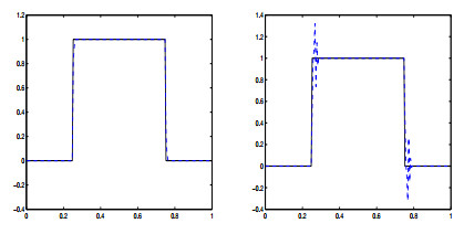
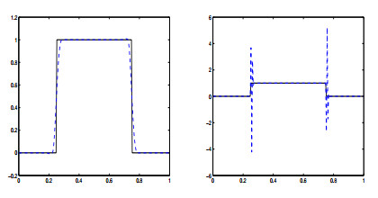
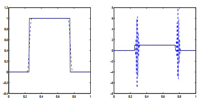
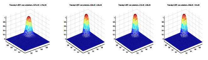
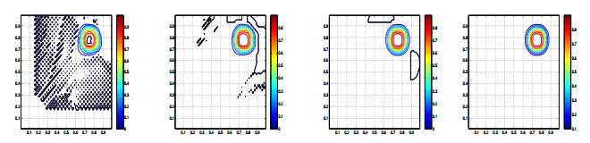
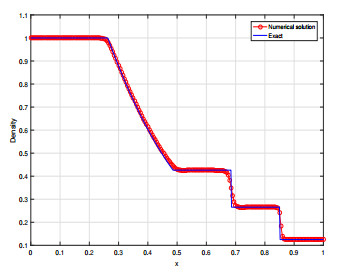
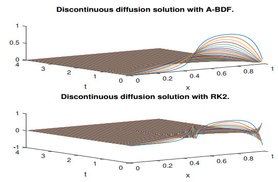
Physical constraints must be taken into account in solving partial differential equations (PDEs) in modeling physical phenomenon time evolution of chemical or biological species. In other words, numerical schemes ought to be devised in a way that numerical results may have the same qualitative properties as those of the theoretical results. Methods with monotonicity preserving property possess a qualitative feature that renders them practically proper for solving hyperbolic systems. The need for monotonicity signifies the essential boundedness properties necessary for the numerical methods. That said, for many linear multistep methods (LMMs), the monotonicity demands are violated. Therefore, it cannot be concluded that the total variations of those methods are bounded. This paper investigates monotonicity, especially emphasizing the stepsize restrictions for boundedness of A-BDF methods as a subclass of LMMs. A-stable methods can often be effectively used for stiff ODEs, but may prove inefficient in hyperbolic equations with stiff source terms. Numerical experiments show that if we apply the A-BDF method to Sod's problem, the numerical solution for the density is sharp without spurious oscillations. Also, application of the A-BDF method to the discontinuous diffusion problem is free of temporal oscillations and negative values near the discontinuous points while the SSP RK2 method does not have such properties.
Citation: Dumitru Baleanu, Mohammad Mehdizadeh Khalsaraei, Ali Shokri, Kamal Kaveh. On the boundedness stepsizes-coefficients of A-BDF methods[J]. AIMS Mathematics, 2022, 7(2): 1562-1579. doi: 10.3934/math.2022091
Physical constraints must be taken into account in solving partial differential equations (PDEs) in modeling physical phenomenon time evolution of chemical or biological species. In other words, numerical schemes ought to be devised in a way that numerical results may have the same qualitative properties as those of the theoretical results. Methods with monotonicity preserving property possess a qualitative feature that renders them practically proper for solving hyperbolic systems. The need for monotonicity signifies the essential boundedness properties necessary for the numerical methods. That said, for many linear multistep methods (LMMs), the monotonicity demands are violated. Therefore, it cannot be concluded that the total variations of those methods are bounded. This paper investigates monotonicity, especially emphasizing the stepsize restrictions for boundedness of A-BDF methods as a subclass of LMMs. A-stable methods can often be effectively used for stiff ODEs, but may prove inefficient in hyperbolic equations with stiff source terms. Numerical experiments show that if we apply the A-BDF method to Sod's problem, the numerical solution for the density is sharp without spurious oscillations. Also, application of the A-BDF method to the discontinuous diffusion problem is free of temporal oscillations and negative values near the discontinuous points while the SSP RK2 method does not have such properties.

| [1] | F. A. Aliev, V. B. Larin, N. Velieva, K. Gasimova, S. Faradjova, Algorithm for solving the systems of the generalized Sylvester-transpose matrix equations using LMI, TWMS J. Pure Appl. Math., 10 (2019), 239–245. |
| [2] | A. F. Aliev, N. A. Aliev, M. M. Mutallimov, A. A. Namazov, Algorithm for solving the identification problem for determining the fractional-order derivative of an oscillatory system, Appl. Comput. Math., 19 (2020), 415–442. |
| [3] | A. Ashyralyev, D. Agirseven, R. P. Agarwal, Stability estimates for delay parabolic differential and difference equations, Appl. Comput. Math., 19 (2020), 175–204. |
| [4] | A. Ashyralyev, A. S. Erdogan, S. N. Tekalan, An investigation on finite difference method for the first order partial differential equation with the nonlocal boundary condition, Appl. Comput. Math., 18 (2019), 247–260. |
| [5] | P. Assari, M. Dehghan, The numerical solution of nonlinear weakly singular fredholm integral equations based on the dual-chebyshev wavelets, Appl. Comput. Math., 19 (2020), 3–19. |
| [6] | M. E. Aydin, A. Erdur, M. Ergut, Affine factorable surfaces in isotropic spaces, TWMS J. Pure Appl. Math., 19 (2020), 72–88. |
| [7] | J. C. Butcher, Numerical methods for ordinary differential equations, Wiley, 2003. doi: 10.1002/0470868279. |
| [8] | W. Chen, W. X. Wu, Z. D. Teng, Complete dynamics in a nonlocal dispersal two-strain siv epidemic model with vaccinations and latent delays, Appl. Comput. Math., 19 (2020), 360–391. |
| [9] |
C. Huang, Strong stability preserving hybrid methods, Appl. Numer. Math., 59 (2009), 891–904. doi: 10.1016/j.apnum.2008.03.030. doi: 10.1016/j.apnum.2008.03.030

|
| [10] |
Y. Cui, M. Wisla, Monotonicity properties and solvability of dominated best approximation problem in Orlicz spaces equipped with s-norms, RACSAM 115, 198 (2021). doi: 10.1007/s13398-021-01139-8. doi: 10.1007/s13398-021-01139-8
|
| [11] | J. E. Golanbar, N. Aliev, M. Jahanshahi, Transportation of a BVP including generalized cauchyriemann equation to fredholm integral equation, TWMS J. Pure Appl. Math., 11 (2020), 30–42. |
| [12] | A. Erem, I. Bayramoglu, Bivariate general random threshold models and exceedance statistics, TWMS J. Pure Appl. Math., 11 (2020), 189–203. |
| [13] |
C. Fredebul, A-BDF: A generalization of the backward differentiation formula, SIAM J. Numer. Anal., 35 (1998), 1917–1938. doi: 10.1137/S0036142996306217. doi: 10.1137/S0036142996306217
|
| [14] | S. Gottlieb, Z. J. Grant, J. Hu, R. Shu, High order strong stability preserving multi-derivative implicit and IMEX Runge-Kutta methods with asymptotic preserving properties, 2021. Available from: https://arXiv.org/abs/2102.11939. |
| [15] | T. Gadjiev, S. Aliev, S. Galandarova, A priori estimates for solutions to Dirichlet boundary value problems for polyharmonic equations in generalized Morrey spaces, TWMS J. Pure Appl. Math., 9 (2018), 231–242. |
| [16] | A. Golbabai, O. Nikan, M. Molavi-Arabshahi, Numerical approximation of time fractional advection-dispersion model arising from solute transport in rivers, TWMS J. Pure Appl. Math., 10 (2019), 117–131. |
| [17] |
S. Gottlieb, D. I. Ketcheson, C. W. Shu, High order strong stability preserving time discretizations, J. Sci. Comput., 38 (2009), 251–289. doi: 10.1007/s10915-008-9239-z. doi: 10.1007/s10915-008-9239-z
|
| [18] |
Y. Hadjimichael, D. I. Ketcheson, Strong-stability-preserving additive linear multistep methods, Math. Comp., 87 (2018), 2295–2320. doi: 10.1090/mcom/3296. doi: 10.1090/mcom/3296
|
| [19] |
Y. Hadjimichael, D. I. Ketcheson, L. Loczi, A. Nemeth, Strong stability preserving explicit linear multistep methods with variable step size, SIAM J. Numer. Anal., 54 (2016), 2799–2832. doi: 10.1137/15M101717X. doi: 10.1137/15M101717X
|
| [20] | E. Hairer, S. P. Norsett, G. Wanner, Solving ordinary differential equations i: Nonstiff problems, 2 Eds., Berlin: Springer, 1993. doi: 10.1007/978-3-540-78862-1. |
| [21] |
A. Harten, High resolution schemes for hyperbolic conservation laws, J. Comput. Phys., 49 (1983), 357–393. doi: 10.1016/0021-9991(83)90136-5. doi: 10.1016/0021-9991(83)90136-5
|
| [22] |
J. Huang, C. W. Shu, Bound-preserving modified exponential Runge-Kutta discontinuous Galerkin methods for scalar hyperbolic equations with stiff source terms, J. Comput. Phys., 361 (2018), 111–135. doi: 10.1016/j.jcp.2018.01.051. doi: 10.1016/j.jcp.2018.01.051
|
| [23] |
J. Huang, C. W. Shu, A second-order asymptotic-preserving and positivity-preserving discontinuous Galerkin scheme for the Kerr-Debye model, Math. Models Methods Appl. Sci., 27 (2017), 549–579. doi: 10.1142/S0218202517500099. doi: 10.1142/S0218202517500099
|
| [24] |
W. Hundsdorfer, S. J. Ruuth, On monotonicity and boundedness properties of linear multistep methods, Math. Comp., 75 (2006), 655–672. doi: 10.1090/S0025-5718-05-01794-1. doi: 10.1090/S0025-5718-05-01794-1
|
| [25] |
W. Hundsdorfer, A. Mozartova, M. N. Spijker, Stepsize restrictions for boundedness and monotonicity of multistep methods, J. Sci. Comput., 50 (2012), 265–286. doi:10.1007/s10915-011-9487-1. doi: 10.1007/s10915-011-9487-1
|
| [26] | W. Hundsdorfer, J. G. Verwer, Numerical solution of time-dependent advection-diffusion-reaction equation, Springer Series in Computational Mathematics, Vol. 33, Berlin: Springer, 2003. doi: 10.1007/978-3-662-09017-6. |
| [27] | N. S. Iskenderov, S. I. Allahverdiyeva, An inverse boundary value problem for the boussinesq-love equation with nonlocal integral condition, TWMS J. Pure Appl. Math., 11 (2020), 226–237. |
| [28] | I. S. Jabbarov, G. K. Hasanova, Estimation of areas on some surfaces defined by the system of equations, TWMS J. Pure Appl. Math., 11 (2020), 89–99. |
| [29] | S. Khan, S. A. Wani, M. Riyasat, Study of generalized legendre-appell polynomials via fractional operators, TWMS J. Pure Appl. Math., 11 (2020), 144–156. |
| [30] |
F. Khodadosti, J. Farzi, M. M. Khalsaraei, Monotonicity-preserving splitting schemes for solving balance laws, Iran. J. Numer. Anal. Optim., 11 (2021), 73–94. doi: 10.22067/IJNAO.2021.11328.0. doi: 10.22067/IJNAO.2021.11328.0
|
| [31] |
F. Khodadosti, J. Farzi, M. M. Khalsaraei, Monotonicity-preserving laxwendroff scheme for solving scalar hyperbolic conservation laws, Bull. Iran. Math. Soc., 2021. doi: 10.1007/s41980-020-00524-0. doi: 10.1007/s41980-020-00524-0
|
| [32] | B. Koren, A robust upwind discretization for advection, diffusion and source terms, In: C. B. Vreugdenhil, B. Koren, Numerical methods for advection-difusion problems, Notes on Numerical Fluid Mechanics, Vieweg, Braunschweig, 45 (1993), 117–138. |
| [33] | [10.1016/0010-4655(74)90093-9] J. D. Lambert, Computational method in ordinary differential equation, John Wiley, 1972. doi: 10.1016/0010-4655(74)90093-9. |
| [34] |
B. Lees, L. Taggi, Site-monotonicity properties for reflection positive measures with applications to quantum spin systems, J. Stat. Phys., 183 (2021), 38. doi:10.1007/s10955-021-02778-2. doi: 10.1007/s10955-021-02778-2
|
| [35] |
H. W. J. Lenferink, Contractivity preserving explicit linear multistep methods, Numer. Math., 55 (1989), 213–223. doi: 10.1007/BF01406515. doi: 10.1007/BF01406515
|
| [36] | R. J. LeVeque, Finite volume methods for hyperbolic problems, Cambridge University Press, 2002. doi: 10.1017/CBO9780511791253. |
| [37] | N. I. Mahmudov, I. T. Huseynov, N. A. Aliev, F. A. Aliev, Analytical approach to a class of bagley-torvik equations, TWMS J. Pure Appl. Math., 11 (2020), 238–258. |
| [38] |
M. M. Khalsaraei, An improvement on the positivity results for 2-stage explicit Runge-Kutta methods, J. Comput. Appl. Math., 235 (2010) 137–143. doi: 10.1016/j.cam.2010.05.020. doi: 10.1016/j.cam.2010.05.020
|
| [39] | M. M. Khalsaraei, F. Khodadosti, 2-stage explicit total variation diminishing preserving Runge-Kutta methods, Comput. Methods Differ. Equ., 1 (2013), 30–38. |
| [40] | M. M. Khalsaraei, F. Khodadoosti, A new total variation diminishing implicit nonstandard finite difference scheme for conservation laws, Comput. Methods Differ. Equ., 2 (2014), 91–98. |
| [41] |
M. M. Khalsaraei, A. Shokri, A new explicit singularly P-stable four-step method for the numerical solution of second order IVPs, Iranian J. Math. Chem., 11 (2020), 17–31. doi:10.22052/IJMC.2020.207671.1472. doi: 10.22052/IJMC.2020.207671.1472
|
| [42] | M. M. Khalsaraei, A. Shokri, The new classes of high order implicit six-step P-stable multiderivative methods for the numerical solution of Schrödinger equation, Appl. Comput. Math., 19 (2020), 59–86. |
| [43] |
M. M. Khalsaraei, A. Shokri, M. Molayi, The new high approximation of stiff systems of first ordinary IVPs arising from chemical reactions by k-step L-stable hybrid methods, Iranian J. Math. Chem., 10 (2019), 181–193. doi:10.22052/IJMC.2018.111016.1335. doi: 10.22052/IJMC.2018.111016.1335
|
| [44] | N. Moshtaghi, A. Saadatmandi, Numerical solution for diffusion equations with distributed-order in time based on Sinc-Legendre collocation method, Appl. Comput. Math., 19 (2020), 317–355. |
| [45] | S. Noeiaghdam, D. Sidorov, V. Sizikov, N. Sidorov, Control of accuracy of Taylor-Collocation method to solve the weakly regular Volterra integral equations of the first kind by using the Cestac method, Appl. Comput. Math., 19 (2020), 87–105. |
| [46] | Z. Odibat, Fractional power series solutions of fractional differential equations by using generalized Taylor series, Appl. Comput. Math., 19 (2020), 47–58. |
| [47] |
C. W. Shu, Total-variation-diminishing time discretizations, SIAM J. Sci. Stat. Comput., 9 (1988), 1073–1084. doi: 10.1137/0909073. doi: 10.1137/0909073
|
| [48] | C. W. Shu, Essentially non-oscillatory and weighted essentially non-oscillatory schemes for hyperbolic conservation laws, In: A. Quarteroni, Advanced numerical approximation of nonlinear Hyperbolic equations, Berlin: Springer, 1998. doi: 10.1007/BFb0096355. |
| [49] |
C. W. Shu, S. Osher, Efficient implementation of essetially non-oscillatory shock-capturing schemes, J. Comput. Phys., 77 (1988), 439–471. doi: 10.1016/0021-9991(88)90177-5. doi: 10.1016/0021-9991(88)90177-5
|
| [50] |
M. N. Spijker, Stepsize conditions for general monotonicity in numerical initial value problems, SIAM J. Numer. Anal., 45 (2007), 1226–1245. doi: 10.1137/060661739. doi: 10.1137/060661739
|
| [51] |
M. N. Spijker, The existence of stepsize-coefficients for boundedness of linear multistep methods, Appl. Numer. Math., 63 (2013), 45–57. doi:10.1016/j.apnum.2012.09.005. doi: 10.1016/j.apnum.2012.09.005
|
| [52] | S. H. Strogatz, Nonlinear dynamics and chaos: With aoolications in physics, biology, chemistry and engineering, CRC Press, 2015. doi: 10.1201/9780429492563. |
| [53] |
Z. Sun, C. W. Shu, Strong stability of explicit runge-kutta time discretizations, SIAM J. Numer. Anal., 57 (2019), 1158–1182. doi: 10.1137/18M122892X. doi: 10.1137/18M122892X
|
| [54] | N. H. Sweilam, A. M. Nagy, A. A. El-Sayed, Sinc-chebyshev collocation method for time-fractional order telegraph equation, Appl. Comput. Math., 19 (2020), 162–174. |
| [55] |
B. Yeager, E. Kubatko, D.Wood, Time step restrictions for strong-stability-preserving multistep rungekutta discontinuous galerkin methods, J. Sci. Comput., 89 (2021), 29. doi: 10.1007/s10915-021-01635-4. doi: 10.1007/s10915-021-01635-4
|
Figures(11) / Tables(3)

Dumitru Baleanu, Mohammad Mehdizadeh Khalsaraei, Ali Shokri, Kamal Kaveh. On the boundedness stepsizes-coefficients of A-BDF methods[J]. AIMS Mathematics, 2022, 7(2): 1562-1579. doi: 10.3934/math.2022091


 DownLoad: