Assessment of health status of tree trunks using ground penetrating radar tomography

Maria Sudakova; Evgeniya Terentyeva; Alexey Kalashnikov; Maria Sudakova; Evgeniya Terentyeva; Alexey Kalashnikov

doi:10.3934/geosci.2021010

AIMS Geosciences

2021, Volume 7, Issue 2: 162-179. doi: 10.3934/geosci.2021010

Previous Article Next Article

Research article Special Issues

Assessment of health status of tree trunks using ground penetrating radar tomography

1.
MSU Lomonosov, geology faculty, seismic department, 119991, GSP-1, 1 Leninskiye Gory, Moscow, Russia
2.
Earth Cryosphere Institute Tyumen Scientific Centre SB RAS, 625000, Maligyna, 86, Tyumen, Russia
3.
Moscow State University of Civil Engineering, 129337, 26, Yaroslavskoye Shosse, Moscow Russia

Received: 30 November 2020 Accepted: 29 March 2020 Published: 08 April 2021

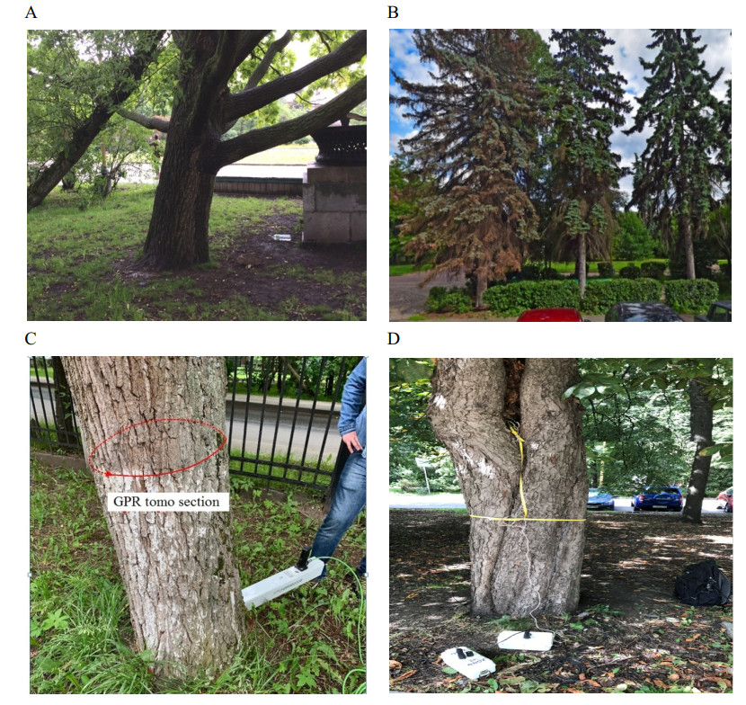
Typical tree health assessment methods are destructive. Non-destructive Ground Penetrating Radar (GPR) technique can provide a diagnostic tool for assessing the health status of live tree trunks based on internal dielectric permittivity distribution. Typical GPR acquisition technique—common-offset—is not helpful in providing robust and high-resolution quantitative results. In the current work we evaluate the capabilities of GPR tomography on locating tree-decays in a number of different tree species, imaging the interval structure of a healthy tree and quantitative estimation of moisture content (MC) based on distribution of dielectric permittivity, directly related to MC. The measurements described in this work were made on the trunks of live trees of different species in different conditions: a "healthy" English oak (Quercus robur), a "dry" Siberian fir (Picea obovata), a Horse chestnut (Castanea dentata) and a European aspen (Populus tremula) with rot inside. The results of the suggested approach were confirmed by resistography. Different parts of the trunk (bark, core, sapwood), as well as healthy and affected areas differ in moisture content, so the method of GPR tomography allowed us to see both the structure of the trunk of a healthy tree, and the presence and dimensions of defects.
- non-destructive testing,
- tree stability,
- wood decay,
- wood moisture content,
- trees monitoring
Citation: Maria Sudakova, Evgeniya Terentyeva, Alexey Kalashnikov. Assessment of health status of tree trunks using ground penetrating radar tomography[J]. AIMS Geosciences, 2021, 7(2): 162-179. doi: 10.3934/geosci.2021010

Related Papers:

Abstract

Typical tree health assessment methods are destructive. Non-destructive Ground Penetrating Radar (GPR) technique can provide a diagnostic tool for assessing the health status of live tree trunks based on internal dielectric permittivity distribution. Typical GPR acquisition technique—common-offset—is not helpful in providing robust and high-resolution quantitative results. In the current work we evaluate the capabilities of GPR tomography on locating tree-decays in a number of different tree species, imaging the interval structure of a healthy tree and quantitative estimation of moisture content (MC) based on distribution of dielectric permittivity, directly related to MC. The measurements described in this work were made on the trunks of live trees of different species in different conditions: a "healthy" English oak (Quercus robur), a "dry" Siberian fir (Picea obovata), a Horse chestnut (Castanea dentata) and a European aspen (Populus tremula) with rot inside. The results of the suggested approach were confirmed by resistography. Different parts of the trunk (bark, core, sapwood), as well as healthy and affected areas differ in moisture content, so the method of GPR tomography allowed us to see both the structure of the trunk of a healthy tree, and the presence and dimensions of defects.

References

[1]	Johnstone D, Moore G, Tausz M, et al. (2010) The measurement of wood decay in landscape trees. Arboric Urban For 36: 121-127.
[2]	Sambuelli L, Socco LV, Godio A, et al. (2003) Ultrasonic, electric and radar measurements for living trees assessment. B Geofis Teor Appl 44: 253-279.
[3]	Rabe C, Ferner D, Fink S, et al. (2004) Detection of decay in trees with stress waves and interpretation of acoustic tomograms. Arboricultural J 28: 3-19. doi: 10.1080/03071375.2004.9747399
[4]	Göcke L, Rust S, Weihs U, et al. (2007) Combining sonic and electrical impedance tomography for the non-destructive testing of trees. Proceedings of 15th international symposium on nondestructive testing of wood. Forest products society. Madison, 31-42.
[5]	Leong EC, Burcham DC, Yok-King F (2012) A purposeful classification of tree decay detection tools. Arboricultural J Int J Urban For 34: 91-115. doi: 10.1080/03071375.2012.701430
[6]	Mattheck CG, Breloer H (1994) Field guide for visual tree assessment (VTA). Arboricultural J Int J Urban For 18: 1-23. doi: 10.1080/03071375.1994.9746995
[7]	Hayes E (2001) Evaluating Tree Defects, Safe trees, 2 Eds., Rochester, 34.
[8]	Luley CL (2005) Wood decay fungi common to living urban trees in the Northeast and Central United States, Naples: Urban Forestry, 61.
[9]	Rinn F, Schweingruber FH, Schiir E (1996) RESISTOGRAPH and X-ray density charts of wood comparative evaluation of drill resistance profiles and X-ray density charts of different wood species. Holzforschung 50: 303-311. doi: 10.1515/hfsg.1996.50.4.303
[10]	Martin T, Günther T (2013) Complex Resistivity Tomography (CRT) for fungus detection on standing oak trees. Eur J For Res 132 : 765-776. doi: 10.1007/s10342-013-0711-4
[11]	Gilbert EA, Smiley ET (2004) Picus sonic tomography for the quantification of decay in white oak (Quercus alba) and hickory (Carya spp.). J Arboric 30: 277-280.
[12]	Wessoly L (1995) Fracture diagnosis of trees. Part 3: Boring is no way for reliable fracture diagnosis. Stadt Und Grün 9: 635-640.
[13]	Hagrey SA (2007) Geophysical imaging of root-zone, trunk, and moisture heterogeneity. J Exp Bot 58: 839-854. doi: 10.1093/jxb/erl237
[14]	Bassuk N, Grabosky J, Mucciardi A, et al. (2011) Ground-penetrating radar accurately locates tree roots in two soil media under pavement. Arboric Urban For 37: 160-166.
[15]	Zhu SP, Huang CL, Su Y, et al. (2014) 3D Ground penetrating radar to detect tree roots and estimate root biomass in the field. Remote Sens 6: 5754-5773. doi: 10.3390/rs6065754
[16]	Satriani A, Loperte A, Proto M, et al. (2010) Building damage caused by tree roots: laboratory experiments of GPR and ERT surveys. Adv Geosci 24: 133-137. doi: 10.5194/adgeo-24-133-2010
[17]	Lorenzo H, Pérez-Gracia V, Novo A, et al. (2010) Forestry applications of ground-penetrating radar. For Syst 19: 5-17.
[18]	Muller W (2003) Timber girder inspection using ground penetrating radar. OR Insight 45: 809-812.
[19]	Pyakurel S (2009) 2D and 3D GPR imaging of wood and fiber reinforced polymer composites. West Virginia University, Morgantown
[20]	Halabe UB, Agrawal S, Gopalakrishnan B (2009) Non-destructive evaluation of wooden logs using ground penetrating radar. Nondestr Test Eval 24: 329-346. doi: 10.1080/10589750802474344
[21]	Colla C (2010) GPR of a timber structural element. Proceedings of 13th international conference on ground penetrating radar, Lecce.
[22]	Rodriguez-Abad I, et al. (2010) Non-destructive methodologies for the evaluation of moisture content in sawn timber structures: ground-penetrating radar and ultrasound techniques. Near Surf Geophys 8: 475-482. doi: 10.3997/1873-0604.2010048
[23]	Jezova J, Lambot S (2019) Influence of bark surface roughness on tree trunk radar inspection. Ground Penetrating Radar 2: 1-25. Available from: https://doi.org/10.26376/GPR2019001.
[24]	Nicolotti G, Socco LV, Martinis R, et al. (2003) Application and comparison of three tomographic techniques for detection of decay in trees. J Arboric 29: 66-78.
[25]	Sudakova MS, Kalashnikov AU, Terentieva EB (2017) GPR tomography as applied to delineation of voids. Construction Unique Build Struct 60: 57.
[26]	Sihvola A (2000) Mixing rules with complex dielectric coefficients. Subsurf Sens Technol Appl 1: 393-415. doi: 10.1023/A:1026511515005
[27]	Huisman JA, Hubbard SS, Redman JD, et al. (2003) Measuring soil water content with ground penetrating radar: a review. Vadose Zone J 2: 476-491. doi: 10.2136/vzj2003.4760
[28]	Hartley I, Hamza MF (2016) Wood: Moisture Content, Hygroscopicity, and Sorption. In: Saleem Hashmi (Editor in chief), Reference Module in Materials Science and Materials Engineering, Oxford: Elsevier.
[29]	Torgovnikov G (1993) Dielectric properties of wood and wood-based materials. Berlin, Heidelberg, New-York: Springer-Verlag, 196.
[30]	Sahin H, Ay N (2004) Dielectric properties of hardwood species at microwave frequencies. J Wood Sci 50: 375-380. doi: 10.1007/s10086-003-0575-1
[31]	Sbartaï, ZM, Lataste JF (2008) Evaluation non-destructive de l'humidité du bois par mesures radar et résistivité électrique. Rapport interne, Université bordeaux 1, US2B, Ghymac.
[32]	Jol HM (2009) Ground penetrating radar theory and applications, Oxford: Elsevier, 523.
[33]	Kabir MF, Khalid KB, Daud WM, et al. (1997) Dielectric properties of rubber wood at microwave frequencies measured with an open-ended coaxial line. Wood Fiber Sci 29: 319-324.
[34]	Afzal MT, Colpits B, Galik K (2003) Dielectric Properties of Softwood Species Measured with an Open-ended Coaxial Probe. In proceedings 8th International IUFRO Wood Drying Conference, Brasvo, Romania, August, 24-29, 2003; 110-115.
[35]	Koubaa A, Perré P, Hutcheon RM, et al. (2008) Complex Dielectric Properties of the Sapwood of Aspen, White Birch, Yellow Birch, and Sugar Maple. Drying Technol 26: 568-578. doi: 10.1080/07373930801944762
[36]	Topp GC, Davis JL, Annan AP (1980) Electromagnetic determination of soil water content: measurements in coaxial transmission lines. Water Resour Res 16: 574-582. doi: 10.1029/WR016i003p00574
[37]	Lin G, Lv JX, Wen J (2014) Research on the relationship between moisture content and the dielectric constant of the tree trunk by the radar wave. Comput Modell New Technol 18: 1171-1175.
[38]	Razafindratsima S, Sbartaï ZM, Demontoux F (2017) Permittivity measurement of wood material over a wide range of moisture content. Wood Sci Technol 51: 1421-1431. doi: 10.1007/s00226-017-0935-4
[39]	Acuna L, Basterra LA, Casado M, et al. (2011) Application of resistograph to obtain the density and to differentiate wood species. Mater Construcc 61: 451-464. doi: 10.3989/mc.2010.57610

Reader Comments

your name:*

Email:*
© 2021 the Author(s), licensee AIMS Press. This is an open access article distributed under the terms of the Creative Commons Attribution License (http://creativecommons.org/licenses/by/4.0)