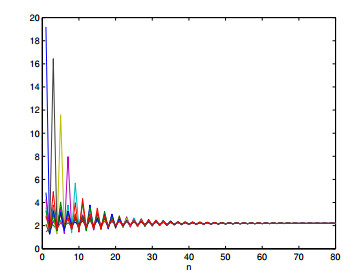
Figure 1.
The plot of system (23) with A=1.2>1 .
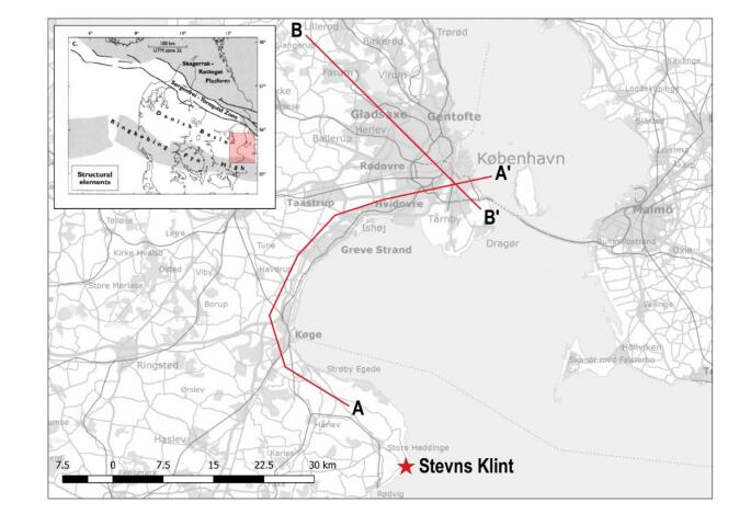
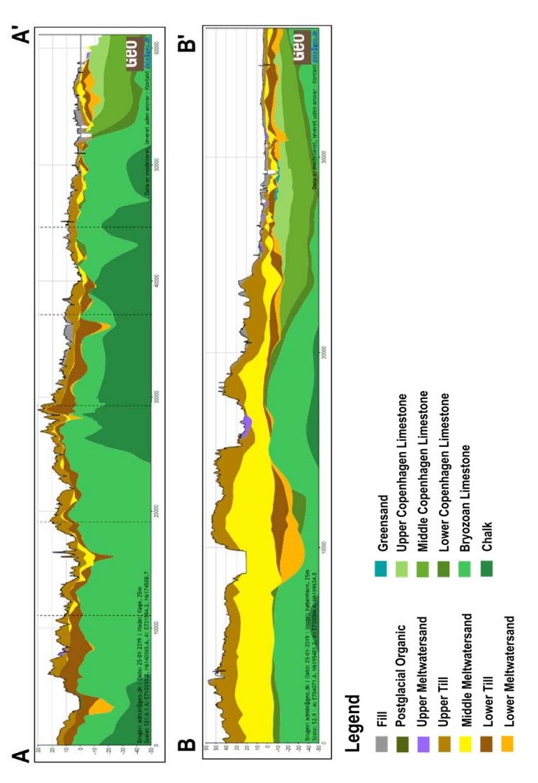
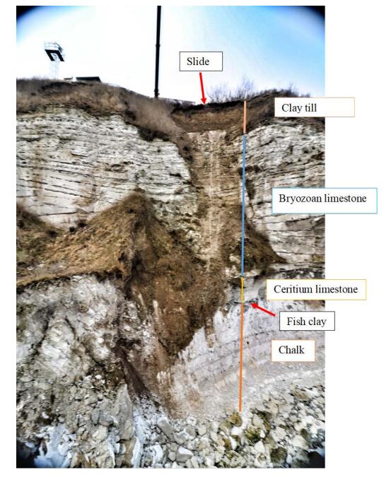
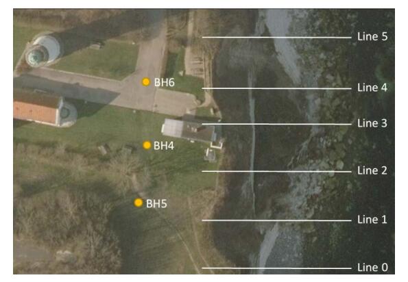
Citation: Nataša Katić, Joakim S. Korshøj, Helle F. Christensen. Bryozoan limestone experience—the case of Stevns Klint[J]. AIMS Geosciences, 2019, 5(2): 163-183. doi: 10.3934/geosci.2019.2.163
| [1] | Amira Khelifa, Yacine Halim . Global behavior of P-dimensional difference equations system. Electronic Research Archive, 2021, 29(5): 3121-3139. doi: 10.3934/era.2021029 |
| [2] | Najmeddine Attia, Ahmed Ghezal . Global stability and co-balancing numbers in a system of rational difference equations. Electronic Research Archive, 2024, 32(3): 2137-2159. doi: 10.3934/era.2024097 |
| [3] | Bin Wang . Random periodic sequence of globally mean-square exponentially stable discrete-time stochastic genetic regulatory networks with discrete spatial diffusions. Electronic Research Archive, 2023, 31(6): 3097-3122. doi: 10.3934/era.2023157 |
| [4] | Tran Hong Thai, Nguyen Anh Dai, Pham Tuan Anh . Global dynamics of some system of second-order difference equations. Electronic Research Archive, 2021, 29(6): 4159-4175. doi: 10.3934/era.2021077 |
| [5] | Wedad Albalawi, Fatemah Mofarreh, Osama Moaaz . Dynamics of a general model of nonlinear difference equations and its applications to LPA model. Electronic Research Archive, 2024, 32(11): 6072-6086. doi: 10.3934/era.2024281 |
| [6] | Merve Kara . Investigation of the global dynamics of two exponential-form difference equations systems. Electronic Research Archive, 2023, 31(11): 6697-6724. doi: 10.3934/era.2023338 |
| [7] | Qianhong Zhang, Shirui Zhang, Zhongni Zhang, Fubiao Lin . On three-dimensional system of rational difference equations with second-order. Electronic Research Archive, 2025, 33(4): 2352-2365. doi: 10.3934/era.2025104 |
| [8] | Chang Hou, Hu Chen . Stability and pointwise-in-time convergence analysis of a finite difference scheme for a 2D nonlinear multi-term subdiffusion equation. Electronic Research Archive, 2025, 33(3): 1476-1489. doi: 10.3934/era.2025069 |
| [9] | Nouressadat Touafek, Durhasan Turgut Tollu, Youssouf Akrour . On a general homogeneous three-dimensional system of difference equations. Electronic Research Archive, 2021, 29(5): 2841-2876. doi: 10.3934/era.2021017 |
| [10] | Ling Xue, Min Zhang, Kun Zhao, Xiaoming Zheng . Controlled dynamics of a chemotaxis model with logarithmic sensitivity by physical boundary conditions. Electronic Research Archive, 2022, 30(12): 4530-4552. doi: 10.3934/era.2022230 |
Difference equations are the essentials required to understand even the simplest epidemiological model: the SIR-susceptible, infected, recovered-model. This model is a compartmental model, which results in the basic difference equation used to measure the actual reproduction number. It is this basic model that helps us determine whether a pathogen is going to die out or whether we end up having an epidemic. This is also the basis for more complex models, including the SVIR, which requires a vaccinated state, which helps us to estimate the probability of herd immunity.
There has been some recent interest in studying the qualitative analysis of difference equations and system of difference equations. Since the beginning of nineties there has be considerable interest in studying systems of difference equations composed by two or three rational difference equations (see, e.g., [4,5,6,2,8,9,11,10,14,15,17,19,20] and the references therein). However, given the multiplicity of factors involved in any epidemic, it will be important to study systems of difference equations composed by many rational difference equations, which is what we will do in this paper.
In [2], Devault et al. studied the boundedness, global stability and periodic character of solutions of the difference equation
| xn+1=p+xn−mxn | (1) |
where
In [20], Zhang et al. investigated the behavior of the following symmetrical system of difference equations
| xn+1=A+yn−myn,yn+1=A+xn−mxn | (2) |
where the parameter
Complement of the work above, in [8], Gümüş studied the global asymptotic stability of positive equilibrium, the rate of convergence of positive solutions and he presented some results about the general behavior of solutions of system (2). Our aim in this paper is to generalize the results concerning equation (1) and system (2) to the system of
| x(1)n+1=A+x(2)n−mx(2)n,x(2)n+1=A+x(3)n−mx(3)n,…,x(p)n+1=A+x(1)n−mx(1)n,n,m,p∈N0 | (3) |
where
The remainder of the paper is organized as follows. In Section (2), we introduce some definitions and notations that will be needed in the sequel. Moreover, we present, in Theorem (2.4), a result concerning the linearized stability that will be useful in the main part of the paper. Section (3) discuses the behavior of positive solutions of system (3) via semi-cycle analysis method. Furthermore, Section (4) is devoted to study the local stability of the equilibrium points and the asymptotic behavior of the solutions when
In this section we recall some definitions and results that will be useful in our investigation, for more details see [3,7,14,13].
Definition 2.1. (see, [14]) A 'string' of sequential terms
A 'string' of sequential terms
A 'string' of sequential terms
A 'string' of sequential terms
Definition 2.2. (see, [14]) A function
| (x(i)μ−¯x(i))(x(i)μ−¯x(i))≤0,i=1,2,…,p. |
We say that a solution
Let
| f(i):Ik+11×Ik+12×…×Ik+1p→Ik+1i,i=1,2,…,p, |
where
| {x(1)n+1=f(1)(x(1)n,x(1)n−1,…,x(1)n−k,x(2)n,x(2)n−1,…,x(2)n−k,…,x(p)n,x(p)n−1,…,x(p)n−k)x(2)n+1=f(2)(x(1)n,x(1)n−1,…,x(1)n−k,x(2)n,x(2)n−1,…,x(2)n−k,…,x(p)n,x(p)n−1,…,x(p)n−k)⋮x(p)n+1=f(p)(x(1)n,x(1)n−1,…,x(1)n−k,x(2)n,x(2)n−1,…,x(2)n−k,…,x(p)n,x(p)n−1,…,x(p)n−k) | (4) |
where
Define the map
| F:I(k+1)1×I(k+1)2×…×I(k+1)p⟶I(k+1)1×I(k+1)2×…×I(k+1)p |
by
| F(W)=(f(1)0(W),f(1)1(W),…,f(1)k(W),f(2)0(W),f(2)1(W),…, |
| …,f(2)k(W),…,f(p)0(W),f(p)1(W),…,f(p)k(W)), |
where
| W=(u(1)0,u(1)1,…,u(1)k,u(2)0,u(2)1,…,u(2)k,…,u(p)0,u(p)1,…,u(p)k)T, |
| f(i)0(W)=f(i)(W),f(i)1(W)=u(i)0,…,f(i)k(W)=u(i)k−1,i=1,2,…,p. |
Let
| Wn=(x(1)n,x(1)n−1,…,x(1)n−k,x(2)n,x(2)n−1,…,x(2)n−k,…,x(p)n,x(p)n−1,…,x(p)n−k)T. |
Then, we can easily see that system (4) is equivalent to the following system written in vector form
| Wn+1=F(Wn),n∈N0. | (5) |
Definition 2.3. (see, [13]) Let
| Xn+1=F(Xn)=BXn |
where
Theorem 2.4. (see, [13])
1. If all the eigenvalues of the Jacobian matrix
2. If at least one eigenvalue of the Jacobian matrix
In this section, we discuss the behavior of positive solutions of system (3) via semi-cycle analysis method. It is easy to see that system (3) has a unique positive equilibrium point
Lemma 3.1. Let
Proof. Suppose that
| x(j)n0<A+1≤x(j)n0+1 or x(j)n0+1<A+1≤x(j)n0,j=1,2,…,p. |
We suppose the first case, that is,
| x(j)n0<A+1≤x(j)n0+m,j=1,2,…,p. |
So, we get from system (3)
| x(j)n0+m+1=A+x(j+1)mod(p)n0x(j+1)mod(p)n0+m<A+1,j=1,2,…,p. |
The Lemma is proved.
Lemma 3.2. Let
Proof. Assume that there exists
| x(j)n0,x(j)n0+2,…,x(j)n0+m−1<A+1≤x(j)n0+1,x(j)n0+3,…,x(j)n0+m,j=1,2,…,p, | (6) |
or
| x(j)n0+1,x(j)n0+3,…,x(j)n0+m<A+1≤x(j)n0,x(j)n0+2,…,x(j)n0+m−1,j=1,2,…,p. | (7) |
We will prove the case (6). The case (7) Is identical and will not be included. According to system (3) we obtain
| x(j)n0+m+1=A+x(j+1)mod(p)n0x(j+1)mod(p)n0+m<A+1,j=1,2,…,p, |
and
| x(j)n0+m+2=A+x(j+1)mod(p)n0+1x(j+1)mod(p)n0+m+1>A+1,j=1,2,…,p, |
The result proceeds by induction. Thus, the proof is completed.
Lemma 3.3. System (3) has no nontrivial periodic solutions of (not necessarily prime) period
Proof. Suppose that
| (α(1)1,α(2)1,…,α(p)1),(α(1)2,α(2)2,…,α(p)2),…,(α(1)m,α(2)m,…,α(p)m),(α(1)1,α(2)1,…,α(p)1),… |
is a
| (x(1)n−m,x(2)n−m,…,x(p)n−m)=(x(1)n,x(2)n,…,x(p)n),n≥0. |
So, the equilibrium solution
Lemma 3.4. All non-oscillatory solutions of system (3) converge to the equilibrium
Proof. We assume there exists non-oscillatory solutions of system (3). We will prove this lemma for the case of a single positive semi-cycle, the situation is identical for a single negative semi-cycle, so it will be omitted. Assume that
| x(j)n+1=A+x(j+1)mod(p)n−mx(j+1)mod(p)n≥A+1,j=1,2,…,p, |
So, we get
| A+1≤x(j)n≤x(j)n−m,n≥0,j=1,2,…,p | (8) |
From (8), there exists
| limn→+∞x(j)nm+i=δ(j)i. |
Hence,
| (δ(1)0,δ(2)0,…,δ(p)0),(δ(1)1,δ(2)1,…,δ(p)1),…,(δ(1)m−1,δ(2)m−1,…,δ(p)m−1) |
is a periodic solution of (not necessarily prime period) period
Theorem 4.1. Suppose
ⅰ): If
| limn→+∞x(j)2n=+∞,limn→+∞x(j)2n+1=A. |
ⅱ): If
| limn→+∞x(j)2n=A,limn→+∞x(j)2n+1=+∞. |
Proof. (ⅰ): From (3), for
| x(i)1=A+x(i+1)mod(p)−mx(i+1)mod(p)0<A+1x(i+1)mod(p)0<A+(1−A)=1,x(i)2=A+x(i+1)mod(p)1−mx(i+1)mod(p)1>A+x(i+1)mod(p)1−m>x(i+1)mod(p)1−m>11−A. |
By induction, for n
| x(i)2n−1<1,x(i)2n>11−A. | (9) |
So, from (3) and (9), we have
| x(i)2n=A+x(i+1)mod(p)2n−1−mx(i+1)mod(p)2n−1>A+x(i+1)mod(p)2n−1−m>2A+x(i+1)mod(p)2n−3−m>3A+x(i+1)mod(p)2n−5−m>⋯ |
So
| x(i)2n>nA+x(i+1)mod(p)0. | (10) |
By limiting the inequality (10), we get
| limn→∞x(i)2n=∞. | (11) |
On the other hand, from(3), (9) and (11), we get
| limn→∞x(i)2n+1=limn→∞(A+x(i+1)mod(p)2n−mx(i+1)mod(p)2n)=A. |
(ⅱ): The proof is similar to the proof of (ⅰ).
Open Problem. Investigate the asymptotic behavior of the system (3) when
Lemma 4.2. Suppose
Proof. Let
| x(j)i∈[L,LL−1],i=1,2,…,m+1,j=1,2,…,p, |
where
| L=min{α,ββ−1}>1,α=min1≤j≤m+1{x(1)j,x(2)j,…,x(p)j}, |
| β=max1≤j≤m+1{x(1)j,x(2)j,…,x(p)ji}. |
So, we get
| L=1+LL/(L−1)≤x(j)m+2=1+x(j+1)mod(p)1x(j+1)mod(p)m+1≤LL−1, |
thus, the following is obtained
| L≤x(j)m≤LL−1. |
By induction, we get
| x(j)i∈[L,LL−1],j=1,2,…,p,i=1,2,… | (12) |
Theorem 4.3. Suppose
| lim infn→+∞x(i)n=lim infn→+∞x(j)n,i,j=1,2,…,p,lim supn→+∞x(i)n=lim supn→+∞x(j)n,i,j=1,2,…,p. |
Proof. From (12), we can set
| Li=limn→∞supx(i)n,mi=limn→∞infx(i)n,i=1,2,…,p. | (13) |
We first prove the theorem for
| L1≤1+L2m2,L2≤1+L1m1,m1≥1+m2L2,m2≥1+m2L2, |
which implies
| L1m2≤m2+L2≤m1L2≤m1+L1≤m2L1 |
thus, the following equalities are obtained
| m2+L2=m1+L1,L1m2=m1L2. |
So, we get that
| Li=Lj,mi=mj,i,j=1,2,…,p−1, |
From system (3), we have
| Lp−1≤1+Lpmp,Lp≤1+Lp−1mp−1,mp−1≥1+mpLp,mp≥1+mpLp, |
hence, we get
| Lp−1mp≤mp+Lp≤mp−1Lp≤mp−1+Lp−1≤mpLp−1, |
consequently, the following equalities are obtained
| mp+Lp=mp−1+Lp−1,Lp−1mp=mp−1Lp. |
So, we get that
Theorem 4.4. Assume that
Proof. The linearized equation of system (3) about the equilibrium point
| Xn+1=BXn |
where
| B=(JAOO…OOOJAO…OOOOJA…OO⋮⋮⋮⋮⋮⋮OOOO…JAAOOO…OJ) |
where
| J=(00…0010…00⋮⋮⋱⋮⋮00…10),O=(00…0000…00⋮⋮⋱⋮⋮00…00), | (14) |
| A=(−1A+10…01A+100…00⋮⋱…⋮⋮00…00). | (15) |
Let
| D=diag(d1,d2,…,dpm+p) |
be a diagonal matrix where
| 0<ε<A−1(m+1)(A+1). | (16) |
It is obvious that
| DBD−1=(J(1)A(1)OO…OOOJ(2)A(2)O…OOOOJ(3)A(3)…OO⋮⋮⋮⋮⋮⋮OOOO…J(p−1)A(p−1)A(p)OOO…OJ(p)), |
where
| J(j)=(00…00d(j−1)m+j+1d(j−1)m+j0…00⋮⋮⋱⋮⋮00…d(j−1)m+m+jd(j−1)m+m+j−10),j=0,1,…,p, |
| A(j)=(−1A+1djdjm+j+10…01A+1djdjm+j+100…00⋮⋱…⋮⋮00…00),j=0,1,…,p−1, |
and
| A(p)=(−1A+1d(p−1)m+pd10…01A+1d(p−1)m+pdm+100…00⋮⋱…⋮⋮00…00). |
From
| A(p)=(−1A+1d(p−1)m+pd10…01A+1d(p−1)m+pdm+100…00⋮⋱…⋮⋮00…00). |
Moreover, from
| 1A+1+1(1−(m+1)ε)(A+1)<1(1−(m+1)ε)(A+1)+1(1−(m+1)ε)(A+1)<2(1−(m+1)ε)(A+1)<1. |
It is common knowledge that
| 1A+1+1(1−(m+1)ε)(A+1)<1(1−(m+1)ε)(A+1)+1(1−(m+1)ε)(A+1)<2(1−(m+1)ε)(A+1)<1. |
We have that all eigenvalues of
To prove the global stability of the positive equilibrium, we need the following lemma.
Lemma 4.5. Suppose
Proof. Let
| x(j)i∈[L,LL−A],i=1,2,…,m+1,j=1,2,…,p, |
where
| L=min{α,ββ−1}>1,α=min1≤j≤m+1{x(1)j,x(2)j,…,x(p)j}, |
| β=max1≤j≤m+1{x(1)j,x(2)j,…,x(p)ji}. |
So, we get
| L=A+LL/(L−A)≤x(j)m+2=A+x(j+1)mod(p)1x(j+1)mod(p)m+1≤LL−1, |
thus, the following is obtained
| L≤x(j)m≤LL−1. |
By induction, we get
| x(j)i∈[L,LL−1],j=1,2,…,p,i=1,2,… | (17) |
Theorem 4.6. Assume that
Proof. Let
| limn→∞(x(1)n,x(2)n,…,x(p)n)=(A+1,A+1,…,A+1). |
To do this, we prove that for
| limn→∞x(i)n=A+1. |
From Lemma (4.5), we can set
| Li=limn→∞supx(i)n,mi=limn→∞infx(i)n,i=1,2,…,p. | (18) |
So, from (3) and (13), we have
| Li≤A+L(i+1)mod(p)m(i+1)mod(p),mi≥A+m(i+1)mod(p)L(i+1)mod(p). | (19) |
We first prove the theorem for
| AL1+m1≤L1m2≤Am2+L2,AL2+m2≤L2m1≤Am1+L1. |
So,
| AL1+m1−(Am1+L1)≤Am2+L2−(AL2+m2), |
hence
| (A−1)(L1−m1+L2−m2)≤0, |
since
| L1−m1+L2−m2=0, |
we know that
| ALp+mp≤Lpm1≤Am1+L1,AL1+m1≤L1mp≤Amp+Lp. |
So,
| ALp+mp−(Amp+Lp)≤Am1+L1−(AL1+m1), |
Thus, the following inequality is obtained
| (A−1)(Lp−mp+L1−m1)≤0, |
since
| Li=mi,=1,2,…,p. |
Therefore every positive solution
In this section, we estimate the rate of convergence of a solution that converges to the equilibrium point
| Xn+1=(A+Bn)Xn | (20) |
where
| ‖Bn‖→0, when n→∞ | (21) |
where
Theorem 5.1. (Perron's first Theorem, see [16]) Suppose that condition (21) holds. If
| ρ=limn→+∞‖Xn+1‖‖Xn‖ |
exists and is equal to the modulus of one of the eigenvalues of matrix
Theorem 5.2. (Perron's second Theorem, see [16]) Suppose that condition (21) holds. If
| ρ=limn→+∞(‖Xn‖)1n |
exists and is equal to the modulus of one of the eigenvalues of matrix
Theorem 5.3. Assume that a solution
| en=(e(1)ne(1)n−1⋮e(1)n−m⋮e(p)ne(p)n−1⋮e(p)n−m)=(x(1)n−¯x(1)x(1)n−1−¯x(1)⋮x(1)n−m−¯x(1)⋮x(p)n−¯x(p)x(p)n−1−¯x(p)⋮x(p)n−m−¯x(p)) |
of every solution of system (3) satisfies both of the following asymptotic relations:
| limn→+∞‖en+1‖‖en‖=|λiJF((¯x(1),¯x(2),…,¯x(p)))|,i=1,2,…,m |
| limn→+∞(‖en‖)1n=|λiJF((¯x(1),¯x(2),…,¯x(p)))|,i=1,2,…,m |
where
Proof. First, we will find a system that satisfies the error terms. The error terms are given as
| x(j)n+1−¯x(j)=m∑i=0(j)A(1)i(x(1)n−i−¯x(1))+m∑i=0(j)A(2)i(x(2)n−i−¯x(2))+⋯+m∑i=0(j)A(1)i(x(p)n−i−¯x(p)), | (22) |
for
| e(j)n=x(j)n−¯x(j),j=1,2,…,p |
Then, system (22) can be written as
| e(j)n+1=m∑i=0(j)A(1)ie(1)n−i+m∑i=0(j)A(2)ie(2)n−i+⋯+m∑i=0(j)A(1)ie(p)n−i |
where
| e(j)n+1=m∑i=0(j)A(1)ie(1)n−i+m∑i=0(j)A(2)ie(2)n−i+⋯+m∑i=0(j)A(1)ie(p)n−i |
and the others parameters
If we consider the limiting case, It is obvious then that
| e(j)n+1=m∑i=0(j)A(1)ie(1)n−i+m∑i=0(j)A(2)ie(2)n−i+⋯+m∑i=0(j)A(1)ie(p)n−i |
That is
| e(j)n+1=m∑i=0(j)A(1)ie(1)n−i+m∑i=0(j)A(2)ie(2)n−i+⋯+m∑i=0(j)A(1)ie(p)n−i |
where
| en+1=(A+Bn)en |
where
| A=JF((¯x(1),¯x(2),…,¯x(p)))=(JA(1)nOO…OOOJA(2)nO…OOOOJA(3)n…OO⋮⋮⋮⋮⋮⋮OOOO…JA(p−1)nA(p)nOOO…OJ) |
| Bn=(JAOO…OOOJAO…OOOOJA…OO⋮⋮⋮⋮⋮⋮OOOO…JAAOOO…OJ) |
where
| A(j)n=(α(j)n0…0β(j)n00…00⋮⋱…⋮⋮00…00),j=1,2,…,p. |
and
| en+1=(JAOO…OOOJAO…OOOOJA…OO⋮⋮⋮⋮⋮⋮OOOO…JAAOOO…OJ)(e(1)ne(1)n−1⋮e(1)n−m⋮e(p)ne(p)n−1⋮e(p)n−m) |
and
In this section we will consider several interesting numerical examples to verify our theoretical results. These examples shows different types of qualitative behavior of solutions of the system (3). All plots in this section are drawn with Matlab.
Exemple 6.1. Let
| x(1)n+1=1.2+x(2)n−1x(2)n,x(2)n+1=A+x(3)n−1x(3)n,…,x(10)n+1=1.2+x(1)n−1x(1)n,n∈N0 | (23) |
with
Exemple 6.2. Consider the system (23) with

Exemple 6.3. Consider the system (23) with

Exemple 6.4. Let
| x(1)n+1=A+x(2)n−5x(2)n,x(2)n+1=A+x(3)n−5x(3)n,x(3)n+1=A+x(4)n−5x(4)n,x(4)n+1=A+x(1)n−5x(1)n,n∈N0 | (24) |
with

Exemple 6.5. Consider the system (24) with

Exemple 6.6. Consider the system (24) with

In the paper, we studied the global behavior of solutions of system (3) composed by
The findings suggest that this approach could also be useful for extended to a system with arbitrary constant different parameters, or to a system with a nonautonomous parameter, or to a system with different parameters and arbitrary powers. So, we will give the following some important open problems for difference equations theory researchers.
Open Problem 1. study the dynamical behaviors of the system of difference equations
| x(1)n+1=A1+x(2)n−mx(2)n,x(2)n+1=A2+x(3)n−mx(3)n,…,x(p)n+1=Ap+x(1)n−mx(1)n,n,m,p∈N0 |
where
Open Problem 2. study the dynamical behaviors of the system of difference equations
| x(1)n+1=αn+x(2)n−mx(2)n,x(2)n+1=αn+x(3)n−mx(3)n,…,x(p)n+1=αn+x(1)n−mx(1)n,n,m,p∈N0 |
where
Open Problem 3. study the dynamical behaviors of the system of difference equations
| x(1)n+1=A1+(x(2)n−m)p1(x(2)n)q1,x(2)n+1=A2+(x(3)n−m)p2(x(3)n)q2,…,x(p)n+1=Ap+(x(1)n−m)pp(x(1)n)qp, |
where
This work was supported by Directorate General for Scientific Research and Technological Development (DGRSDT), Algeria.
| [1] | Jackson PG, Steenfelt JS, Foged NN, et al. (2004) Evaluation of Bryozoan limestone properties based on in-situ and laboratory element tests. Geotech Geophys Site Charact 1813–1820. |
| [2] | Foged NN (2008) Rock Mass Characterisation in Limestone. Lecture presented at Dansk Geoteknisk Forening Mode nr. 2 Generalforsamling. (Danish Geotechnical Society Meeting nr. 2 General assembly.) |
| [3] | Foged NN, Hansen SL, Stabell S (2010) Developments in Rock Mass Evaluation of Limestone in Denmark. In: Rock mechanics in the Nordic countries, Norway: Kongberg. |
| [4] | Galsgaard J. (2014) Flint in the Danian København Limestone Formation. (Flint in the Danian Copenhagen Limestone Formation.) Available from: https://www.geo.dk/media/1951/flint-in-the-danian-koebenhavn-limestone-formation_jgalsgaard_2014.pdf |
| [5] | Jakobsen L, Foged NN, Erichsen L, et al. (2015) Face logging in Copenhagen Limestone, Denmark. Proceedings of the XVI ECSMGE Geotechnical Engineering for Infrastructure and Development, 2939–2944. |
| [6] | Hansen SL, Galsgaard J, Foged NN (2015) Rock mass characterization for Copenhagen Metro using face logs. SEE TUNNEL-Promoting tunnelling in SE European region, Presented at: 41st General Assembly and Congress of International Tunneling and Underground Space. |
| [7] | Katić N, Christensen HF (2014). Upscaling elastic moduli in Copenhagen Limestone. In Rock Engineering and Rock Mechanics: Structures in and on Rock Masses: Proceedings of EUROCK 2014, ISRM European Regional Symposium, London: Taylor & Francis Group, 235–240. |
| [8] | Katić N, Christensen HF (2015) Composite Elasticity of Copenhagen Limestone. In Proceedings of the ISRM Regional Symposium EUROCK 2015 & 64th Geomechanics Colloquium-Future Development of Rock Mechanics, Salzburg: Austrian Society for Geomechanics, 451–456. |
| [9] | Vangkilde-Pedersen T, Mielby S, Jakobsen PR, et al. (2011) Kortlægning af kalkmagasiner. GEUS. Geo-vejledning 8. De nationale geologiske undersøgelser for Danmark og Grønland. Ministeriet for klima og energy. (Mapping of limestone reservoirs. GEUS. Geo-guidance 8. National geological investigations for Denmark and Greenland. Ministry of climate and energy.) Available from: gk.geus.info/xpdf/geovejledning_8_kalk_final_net.pdf. |
| [10] |
Bjerager M, Surlyk F (2007) Danian Cool-Water Bryozoan Mounds at Stevns Klint, Denmark–A New Class of Non-Cemented Skeletal Mounds. J Sediment Res 77:634–660. doi: 10.2110/jsr.2007.064

|
| [11] |
Japsen P, Bidstrup T, Lidmar-Berström K (2002) Neogene uplift and erosion of southern Scandinavia induced by the rise of the South Swedish Dome. Geol Soc 196: 183–207. doi: 10.1144/GSL.SP.2002.196.01.12
|
| [12] | Andersen TB, Møgaard MR (2018) Copenhagen Area Overview of the geological conditions in the Copenhagen area and surrounding areas. GeoAtlas Live Documentation. Report 1. Available from: http://wgn.geo.dk/geodata/modeldokumentation/Copenhagen%20_25m_2018-07-12.pdf |
| [13] | Olsen H, Nielsen UT (2002) Logstratigrafisk inddeling af kalken I Københavns-området. In Frederiksen JK, Eriksen FS, Hansen HK, et al., editors. Ingeniørgeologiske forhold i København. Dgf-Bulletin 19, Danish Geotechnical Society. (Logstratigraphical division of limestone in Copenhagen Area. In Frederiksen JK, Eriksen FS, Hansen HK, et al., editors. Engineering-geological conditions in Copenhagen. Dgf-Bulletin 19, Danish Geotechnical Society.) |
| [14] | Damholt T, Surlyk F (2012) Nomination of Stevns Klint for inclusion in the World Heritage List. Østsjællands Museum. Pedersen AS (2011) Rockfalls at Stevns Klint. Landslide hazard assessment based on photogrametrical supported geological analysis of the limestone cliff Stevns Klint in eastern Denmark. Danmarks og Grønlands Geologiske Undersøgelse Rapport 2011/93 (Danmark's and Greenland's Geological Investigaton Report 2011/93). Available from: https://whc.unesco.org/uploads/nominations/1416.pdf. |
| [15] | Mortensen N, Hansen HK, Hansen PB (1999) Malmö Citytunneln.Rock Mechanical Description. Limestone. Malmö (SE). 32p. Report 1, 22 March 1999, Revision 1. DGI job No. 155 16092. Geo archive. |
| [16] | Jørgensen NO (1975) Mg/Sr distribution and diagenesis of Maastrichtian white chalk and Danian bryozoan limestone from Jylland, Denmark. Bull Geol Soc Den 24: 299–325. |
| [17] | Rosenbom A, Jakobsen PR (2000) Kalk, Sprækker og Termografi. Geol Nyt fra GEUS 3: 1–8. (Chalk, Fractures and Thermography. Geol News From GEUS 3: 1–8.) |
| [18] | Surlyk F, Damholt T, Bjerager M (2006) Stevns Klint, Denmark: uppermost Maastrichtian chalk, Cretaceous-Tertiary boundary, and lower Danian bryozoan mound complex, Geological Society of Denmark, 54: 1–48. |
| [19] | Hoek E, Carter TG, Diedrichs MS (2013) Quantification of the Geological Strength Index Chart. 47th US Rock Mechanics/Geomechanics Symposium, 1757–1764. |
| [20] |
Eberli GP, Beachle TG, Anselmetti FS, et al. (2003) Factors controlling elastic properties in carbonate sediments and rocks. Lead Edge 22: 654–660. doi: 10.1190/1.1599691
|
| [21] |
Brigaud B, Vincent B, Durlet C, et al. (2010) Acoustic properties of ancient shallow-marine carbonates: effects of depositional environments and diagenetic processes (Middle Jurassic, Paris basin, France). J Sediment Res 80:791–807. doi: 10.2110/jsr.2010.071
|
| [22] | Bergdahl U, Steenfelt JS (1994) Digest report on strength and deformation properties of Copenhagen limestone, Swedish Geotechnical Institute/Danish Geotechnical Institute, 67. |
Nataša Katić, Joakim S. Korshøj, Helle F. Christensen. Bryozoan limestone experience—the case of Stevns Klint[J]. AIMS Geosciences, 2019, 5(2): 163-183. doi: 10.3934/geosci.2019.2.163

 DownLoad: