
Citation: Thomas Fauchez, Giada Arney, Ravi Kumar Kopparapu, Shawn Domagal Goldman. Explicit cloud representation in the Atmos 1D climate model for Earth and rocky planet applications[J]. AIMS Geosciences, 2018, 4(4): 180-191. doi: 10.3934/geosci.2018.4.180
[1] | John D. Towers . The Lax-Friedrichs scheme for interaction between the inviscid Burgers equation and multiple particles. Networks and Heterogeneous Media, 2020, 15(1): 143-169. doi: 10.3934/nhm.2020007 |
[2] | Boris Andreianov, Frédéric Lagoutière, Nicolas Seguin, Takéo Takahashi . Small solids in an inviscid fluid. Networks and Heterogeneous Media, 2010, 5(3): 385-404. doi: 10.3934/nhm.2010.5.385 |
[3] | Jan Friedrich, Oliver Kolb, Simone Göttlich . A Godunov type scheme for a class of LWR traffic flow models with non-local flux. Networks and Heterogeneous Media, 2018, 13(4): 531-547. doi: 10.3934/nhm.2018024 |
[4] | Caterina Balzotti, Simone Göttlich . A two-dimensional multi-class traffic flow model. Networks and Heterogeneous Media, 2021, 16(1): 69-90. doi: 10.3934/nhm.2020034 |
[5] | Raimund Bürger, Harold Deivi Contreras, Luis Miguel Villada . A Hilliges-Weidlich-type scheme for a one-dimensional scalar conservation law with nonlocal flux. Networks and Heterogeneous Media, 2023, 18(2): 664-693. doi: 10.3934/nhm.2023029 |
[6] | Tong Yan . The numerical solutions for the nonhomogeneous Burgers' equation with the generalized Hopf-Cole transformation. Networks and Heterogeneous Media, 2023, 18(1): 359-379. doi: 10.3934/nhm.2023014 |
[7] | Verónica Anaya, Mostafa Bendahmane, David Mora, Ricardo Ruiz Baier . On a vorticity-based formulation for reaction-diffusion-Brinkman systems. Networks and Heterogeneous Media, 2018, 13(1): 69-94. doi: 10.3934/nhm.2018004 |
[8] | Li-Bin Liu, Limin Ye, Xiaobing Bao, Yong Zhang . A second order numerical method for a Volterra integro-differential equation with a weakly singular kernel. Networks and Heterogeneous Media, 2024, 19(2): 740-752. doi: 10.3934/nhm.2024033 |
[9] | Anya Désilles, Hélène Frankowska . Explicit construction of solutions to the Burgers equation with discontinuous initial-boundary conditions. Networks and Heterogeneous Media, 2013, 8(3): 727-744. doi: 10.3934/nhm.2013.8.727 |
[10] | Jie Gu, Lijuan Nong, Qian Yi, An Chen . Two high-order compact difference schemes with temporal graded meshes for time-fractional Black-Scholes equation. Networks and Heterogeneous Media, 2023, 18(4): 1692-1712. doi: 10.3934/nhm.2023074 |
This paper concerns a one-dimensional model of solid-fluid interaction:
{∂tu+∂xf(u)=K∑k=1λk(h′k(t)−u)δ(x−hk(t)),(x,t)∈R×(0,T):=ΠT,mkhk″(t)=λk(u(hk(t),t)−h′k(t)),t∈(0,T),k=1,…,K,u(x,0)=u0(x),(hk(0),h′k(0))=(hk,0,vk,0),k=1,…,K. | (1.1) |
Here
The fluid velocity is governed by the inviscid Burgers equation
There are some difficulties associated with (1.1), in addition to the well-known ones associated with a nonlinear conservation law. The source terms on the right side of the first equation are nonconservative products of distributions; their meaning is not immediately clear. The differential equations appearing in the second line are coupled to the conservation law. Due to discontinuities in
Notwithstanding these difficulties there has been much progress on the single-particle version of (1.1). A notion of solution has been developed, well-posedness has been proven, and numerical algorithms have been designed whose approximations are known to converge to the unique solution. In this paper we focus on the multiple-particle problem, which has not been studied as thoroughly. We propose a notion of entropy solution suitable for multiple particles, present a Lax-Friedrichs difference scheme for the multiple-particle problem, and prove that the resulting approximations converge to an entropy solution. This is accomplished under the assumption that the particle paths do not intersect except possibly at a set of times whose Lebesgue measure is zero.
Reference [4] developed a unifying framework for the jump conditions that hold across a spatial flux discontinuity for a conservation law with discontinuous flux, using the theory of
Definition 1.1 (the germ
G(λ,c)=(c,c)+{(a,b)∈R2|b=a−λ}∪{(a,b)∈R2|a≥0,b≤0,−λ≤a+b≤λ}. | (1.2) |
Reference [6] gives a definition of entropy solution for the single-particle version of (1.1). The following is a direct generalization of that definition to the multiple-particle problem.
Definition 1.2 (entropy solution).
(ⅰ) Given
(u(hk(t)−,t),u(hk(t)+,t))∈G(λk(t),h′k(t)),k=1,…,K. | (1.3) |
(ⅱ) A function
mkh″k(t)=(12u(hk(t)−,t)2−h′k(t)u(hk(t)−,t))−(12u(hk(t)+,t)2−h′k(t)u(hk(t)+,t)). | (1.4) |
(ⅲ) With the notation
Remark 1. Definition 1.2 requires strong one-sided traces
Assumption 1.1. The initial data satisfies
Above we have used the notation
TV(ρ):=sup{M∑i=1|ρ(ξi)−ρ(ξi−1)|}<∞, |
where the
Theorem 1.3 (Main theorem). The Lax-Friedrichs scheme described in Section 2 produces approximations that converge as the mesh size approaches zero, along a subsequence, to a pair
As mentioned above, there has been significant progress on the single-particle version of (1.1) [1,5,6,7,11]. The study of (1.1) started with reference [11]. Among other things the authors completely solved the Riemann problem for
In reference [5], the authors introduce two finite volume methods for computing approximate solutions. One is a Glimm-like scheme, and the other is a well-balanced scheme that uses nonrectangular space-time cells near the interface. These methods employ random sampling for placing the particle at a mesh interface at each time step. The nonconservative source term is handled by using a certain well-balanced scheme that was analyzed in [7]. They avoid the use of a moving mesh, and also avoid the use of a Riemann solver for the full model. The case of multiple particles is addressed, and is handled via a splitting method.
Reference [14] presents a finite volume scheme that is based on the well-balanced scheme of [5,7], but uses an adaptive stencil as an alternative to using a moving grid. The multiple-particle case is handled by splitting.
Reference [7] proves well-posedness for the problem
ut+(u2/2)x=−λuδ(x),u(x,0)=u0(x). | (1.5) |
This is a simplification of (1.1), but its analysis provides an important step in analyzing the full problem. As mentioned above the germ
Reference [6] proves well-posedness of the model (1.1) for
Reference [1] presents a class of finite volume schemes for (1.1) when
References [2] and [3] concern a generalized version of (1.1) (again, for
Reference [10] specifically deals with a multiple-particle problem. The authors prove well-posedness for a version of (1.1) where the particle paths
Let
{∂tu+∂x(u2/2)=K∑k=1λk(h′k(t)−u)∂xwk,(x,t)∈ΠT,∂twk+h′k(t)∂xwk=0,(x,t)∈ΠT,k=1,…,K,mkhk″(t)=λk(u(hk(t),t)−h′k(t)),t∈(0,T),k=1,…,K,u(x,0)=u0(x),(hk(0),h′k(0))=(hk,0,vk,0),k=1,…,K,wk(x,0)=H(x−hk,0),k=1,…,K. | (1.6) |
Although the splitting approach for multiple particles used in [5] and [14] gives good numerical results, extending the convergence analysis from the single-particle to the multiple-particle problem seems difficult. Various bounds required for convergence are not preserved by the splitting steps. The numerical schemes in those papers are based on the model (1.1). In this paper we instead discretize (1.6), using Lax-Friedrichs differencing for each of the PDEs. The advantage of this approach is that the case of multiple particles is accommodated without splitting. This makes it possible to obtain a number of estimates which taken together give a convergence proof for the multiple-particle model. On the other hand, while the schemes of [1], [5], and [14] give very sharply resolved shocks at the particle locations, our Lax-Friedrichs method results in a substantial amount of smearing. With this in mind, we additionally propose a higher resolution version of the scheme, based on MUSCL processing.
The rest of the paper is organized as follows. In Section 2 we describe the Lax-Friedrichs scheme mentioned above. In Section 3 we prove convergence, modulo a subsequence, of the approximations for
We use a uniform spatial mesh size
xj=jΔx,j∈Z,tn=nΔt,0≤n≤N, | (2.1) |
where the integer
Δ+Qnj=Qnj+1−Qnj,Δ−Qnj=Qnj−Qnj−1,ˆQnj=12(Qnj−1+Qnj+1),Qnmin=infj∈ZQnj,Qnmax=supj∈ZQnj,‖Qn‖∞=supj∈Z|Qnj|. | (2.2) |
Let
infx∈Ijv0(x)≤V0j≤supx∈Ijv0(x),and∑j∈Zχj(x)V0j→v0(x)inL1loc(R)asΔx→0. | (2.3) |
With the notation
We extend
uΔ(x,t)=N∑n=0∑j∈Zχj(x)χn(t)Unj,wΔk(x,t)=N∑n=0∑j∈Zχj(x)χn(t)Wnk,j. | (2.4) |
Similarly,
cΔk(t)=N∑n=0χn(t)cnk,hΔk(t)=N∑n=0χn(t)(hnk+(t−tn)cnk), | (2.5) |
where
Let
{Un+1j=Unj−μΔ−ˉfnj+1/2+K∑k=1λkμ2(cnk−ˆUnj)(Wnk,j+1−Wnk,j−1),Wn+1k,j=Wnk,j−μΔ−ˉgnk,j+1/2,cn+1k=cnk−1mk∑j∈ZΔtλk2(cnk−ˆUnj)(Wnk,j+1−Wnk,j−1),hn+1k=hnk+cnkΔt. | (2.6) |
Here
ˉfnj+1/2=ˉf(Unj+1,Unj)=12((Unj+1)2/2+(Unj)2/2)−q2μ(Unj+1−Unj),ˉgnk,j+1/2=12(cnkWnk,j+1+cnkWnk,j)−q2μ(Wnk,j+1−Wnk,j), | (2.7) |
where
Remark 2. The scheme (2.6) preserves solutions where the fluid velocity and particle velocities are equal to the same constant:
Remark 3. Some explanation of the third equation of (2.6) is in order. Based on the third equation of (1.6), the third equation of (2.6) should be (approximately) equivalent to
cn+1k=cnk−1mkΔtλkcnk+1mkΔtλk˜u(hk(tn),tn), |
where
cn+1k=cnk−1mkΔtλkcnk+1mkΔtλk(1/2)∑j∈ZˆUnj(Wnk,j+1−Wnk,j−1). |
Thus, by defining
˜u(hk(tn),tn):=(1/2)∑j∈ZˆUnj(Wnk,j+1−Wnk,j−1)≈∫Ru(x,tn)δ(x−hk(tn))dx, |
we have the desired approximation
From the first two equations of (1.1) it follows that, at least formally, the total momentum of the system is conserved:
ddt(∫Ru(x,t)dx+K∑k=1mkh′k(t))=0. | (2.8) |
The scheme (2.6) enforces a discrete version of (2.8).
Proposition 1. Assume that there is a
Mn=Δx∑j∈ZUnj+K∑k=1mkcnk. | (2.9) |
The discrete momentum is conserved:
Proof. Multiplying by
Δx∑j∈ZUn+1j=Δx∑j∈ZUnj+∑j∈ZK∑k=1λkΔt2(cnk−ˆUnj)(Wnk,j+1−Wnk,j−1). | (2.10) |
Multiplying the third equation of (2.6) by
K∑k=1mkcn+1k=K∑k=1mkcnk−K∑k=1∑j∈ZΔtλk2(cnk−ˆUnj)(Wnk,j+1−Wnk,j−1). | (2.11) |
The proof is completed by adding (2.10) and (2.11).
Define
Znj=Unj+K∑k=1λkWnk,j,zΔ(x,t)=N∑n=0∑j∈Zχj(x)χn(t)Znj. | (2.12) |
Lemma 2.1.
Zn+1j=Znj−μΔ−ˉf(Znj+1,Znj)+μ2K∑k=1λkˆWnk,j(Znj+1−Znj−1), | (2.13) |
Zn+1j=Znj+12(q−μˆUnj)Δ+Znj−12(q+μˆUnj)Δ−Znj. | (2.14) |
Remark 4. From (1.6) and the definition
∂tz+∂xf(z)=K∑k=1λkwk∂xz. | (2.15) |
Evidently (2.13) is a discretization of (2.15).
Remark 5. It is clear by inspection of either (2.13) or (2.14) that the scheme (2.6) preserves solutions of the form
Proof. Using (2.12) and (2.6) we find that
Zn+1j=Unj−μΔ−ˉfnj+1/2+K∑k=1λkμ2(cnk−ˆUnj)(Wnk,j+1−Wnk,j−1)+K∑k=1λk(Wnk,j−μΔ−ˉgnk,j+1/2)=Znj−μΔ−ˉfnj+1/2+K∑k=1λkμ2(cnk−ˆUnj)(Wnk,j+1−Wnk,j−1)−μK∑k=1λkΔ−ˉgnk,j+1/2. | (2.16) |
Next we use
Δ−ˉfnj+1/2=12ˆUnj(Unj+1−Unj−1)−q2μΔ+Δ−Unj,Δ−ˉgnk,j+1/2=12cnk(Wnk,j+1−Wnk,j−1)−q2μΔ+Δ−Wnk,j. | (2.17) |
Substituting (2.17) into (2.16) and canceling
Zn+1j=Znj−μ2ˆUnj(Unj+1−Unj−1)+q2Δ+Δ−Unj−μ2ˆUnjK∑k=1λk(Wnk,j+1−Wnk,j−1)+q2K∑k=1λkΔ+Δ−Wnk,j=Znj−μ2ˆUnj(Znj+1−Znj−1)+q2Δ+Δ−Znj=Znj−μ2ˆUnj(Δ+Znj+Δ−Znj)+q2(Δ+Znj−Δ−Znj). | (2.18) |
The identity (2.14) is immediate from (2.18).
For the proof of (2.13), we start from the second equality of (2.18) and substitute
Zn+1j=Znj−μ2(ˆZnj−K∑k=1λkˆWnk,j)(Znj+1−Znj−1)+q2Δ+Δ−Znj=Znj−μ2ˆZnj(Znj+1−Znj−1)+μ2(K∑k=1λkˆWnk,j)(Znj+1−Znj−1)+q2Δ+Δ−Znj=Znj−μ2(f(Znj+1)−f(Znj−1))+q2Δ+Δ−Znj+μ2(K∑k=1λkˆWnk,j)(Znj+1−Znj−1). | (2.19) |
The identity (2.13) now follows directly from (2.19).
Let
μmax(max1≤k≤K|c0k|,‖z0‖∞+K∑k=1λk,‖u0‖∞+K∑k=1λk)≤q≤1/2. | (3.1) |
Additionally we assume that
Δt≤mk/λk,k=1,…,K, | (3.2) |
which will be satisfied automatically for
Define
Lemma 3.1. The following properties hold:
z0min≤Znj≤z0max,‖Zn‖∞≤‖z0‖∞, | (3.3) |
u0min−K∑k=1λk≤Unj≤u0max+K∑k=1λk,‖Un‖∞≤‖u0‖∞+K∑k=1λk, | (3.4) |
Wnk,j∈[0,1],Δ+Wnk,j≥0,∑j∈ZΔ+Wnk,j=1, | (3.5) |
|cnk|≤max(|c0k|,‖u0‖∞+K∑k=1λk). | (3.6) |
Proof. The proof is by induction on
μ(‖Zn‖∞+K∑k=1λk)≤q,μ|cnk|≤q,k=1,…,K. | (3.7) |
To prove that (3.3) holds at time step
Zn+1j=Znj+Cnj+1/2Δ+Znj−Dnj−1/2Δ−Znj, | (3.8) |
where
Cnj+1/2=12(q−μˆUnj),Dnj−1/2=12(q+μˆUnj). | (3.9) |
Using
Zn+1j=(1−Cnj+1/2−Dnj−1/2)Znj+Cnj+1/2Znj+1+Dnj−1/2Znj−1. | (3.10) |
From (3.10) it is clear that
Next we prove that (3.5) holds for
Wn+1k,j=(1−αnk−βnk)Wnk,j+αnkWnk,j+1+βnkWnk,j−1, | (3.11) |
where
αnk=12(q−μcnk),βnk=12(q+μcnk). | (3.12) |
By (3.7) we have
Δ+Wn+1k,j=(1−αnk−βnk)Δ+Wnk,j+αnkΔ+Wnk,j+1+βnkΔ+Wnk,j−1. | (3.13) |
Invoking the induction hypothesis again yields
To prove (3.4) holds at
z0min−K∑k=1λkWn+1k,j≤Un+1j≤z0max−K∑k=1λkWn+1k,j. | (3.14) |
It is readily verified that
u0min−K∑k=1λkWn+1k,j≤Un+1j≤u0max+K∑k=1λk−K∑k=1λkWn+1k,j. | (3.15) |
Recalling that
To verify that (3.6) holds for
cn+1k=(1−Δtλk2mk∑j∈Z(Wnk,j+1−Wnk,j−1))cnk+Δtλk2mk∑j∈Z(Wnk,j+1−Wnk,j−1)ˆUnj. | (3.16) |
The induction hypothesis yields
|cn+1k|≤(1−Δtλkmk)|cnk|+Δtλk2mk∑j∈Z(Wnk,j+1−Wnk,j−1)|ˆUnj|≤(1−Δtλkmk)|cnk|+Δtλk2mk∑j∈Z(Wnk,j+1−Wnk,j−1)(‖u0‖∞+K∑k=1λk)=(1−Δtλkmk)|cnk|+Δtλkmk(‖u0‖∞+K∑k=1λk)≤(1−Δtλkmk)max(|c0k|,‖u0‖∞+K∑k=1λk)+Δtλkmk(‖u0‖∞+K∑k=1λk), | (3.17) |
from which the desired inequality follows readily.
Lemma 3.2.
∑j∈Z|Δ+Znj|≤TV(u0)+K∑k=1λk, | (3.18) |
and
∑j∈Z|Δ+Unj|≤TV(u0)+2K∑k=1λk. | (3.19) |
Proof. We claim that the scheme is a so-called Total Variation Decreasing (TVD) scheme with respect to the variable
∑j∈Z|Δ+Zn+1j|≤∑j∈Z|Δ+Znj|. | (3.20) |
To prove the claim we use (3.8). We have shown that
Cnj+1/2+Dnj+1/2=q−μ4(Unj+1+Unj−1)+μ4(Unj+2+Unj)≤q+μ‖Un‖∞≤q+μ(‖u0‖∞+K∑k=1λk)≤2q. | (3.21) |
Here we have used (3.1) to get the last inequality. The desired bound then results by recalling that
∑j∈Z|Δ+Znj|≤∑j∈Z|Δ+Z0j|≤TV(z0). | (3.22) |
It is readily verified using (2.12) that
∑j∈Z|Unj+1−Unj|−K∑k=1λk≤∑j∈Z|Znj+1−Znj|≤∑j∈Z|Unj+1−Unj|+K∑k=1λk. | (3.23) |
Then (3.18) follows from (3.22) and the
Lemma 3.3. The following time continuity estimate holds:
∑j∈Z|Un+1j−Unj|≤B, | (3.24) |
where the constant
Proof. Rearranging the first equation of (2.6), and using (2.17) to rewrite
Un+1j−Unj=12(q−μˆUnj)Δ+Unj−12(q+μˆUnj)Δ−Unj+μ2K∑k=1λk(cnk−ˆUnj)(Wnk,j+1−Wnk,j−1). | (3.25) |
After taking absolute values, applying the triangle inequality, then using the bounds on
∑j∈Z|Un+1j−Unj|≤B1∑j∈Z|Δ+Unj|+B2K∑k=1∑j∈Z|Wnk,j+1−Wnk,j−1|, | (3.26) |
where
Lemma 3.4. The particle velocity approximations satisfy the following bound:
|cn+1k−cnk|≤λkΔtmk(max(|c0k|,‖u0‖∞+K∑k=1λk)+‖u0‖∞+K∑k=1λk). | (3.27) |
Proof.
We start with the third formula of (2.6). Subtracting
\begin{equation} \begin{split} \left|{c_k^{n+1}-c_k^n}\right| & \le {1\over{m_k}}\sum\limits_{j \in \mathbb{Z}} {{\Delta t \lambda_k}\over 2}\left|{c_k^n - \hat{U}_j^n}\right| \left(W^n_{k,j+1}-W^n_{k,j-1} \right)\\ & \le {1\over{m_k}}\sum\limits_{j \in \mathbb{Z}} {{\Delta t \lambda_k}\over 2}\left(\left|{c_k^n}\right| + \left\|{U^n}\right\|_{\infty} \right) \left(W^n_{k,j+1}-W^n_{k,j-1} \right)\\ & = {{\Delta t \lambda_k}\over {m_k}}\left(\left|{c_k^n}\right| + \left\|{U^n}\right\|_{\infty} \right). \end{split} \end{equation} | (3.28) |
The proof of (3.27) is completed using (3.4) and (3.6).
Lemma 3.5. The approximations
Proof. The proof is a standard argument (e.g., the proof of Proposition 2.4 of [1]) using Lemmas 3.1, 3.2, and 3.3 for the
Remark 6. In Sections 5 and 6 we will assume that the particle trajectories do not intersect except possibly on a subset of
In what follows
Lemma 4.1.
\begin{equation} \sum\limits_{j \in \mathbb{Z}} \left|{\Delta_+ W_{k,j}^n}\right| = 1, \quad \sum\limits_{j \in \mathbb{Z}} \left|{W_{k,j}^{n+1}-W_{k,j}^n}\right| \le 1/2. \end{equation} | (4.1) |
Proof. The first part of (4.1) is evident from (3.5). For the second part of (4.1), we write (3.11) in the form
\begin{equation} W_{k,j}^{n+1}-W_{k,j}^n = \alpha_k^n\Delta_+W_{k,j}^n - \beta_k^n \Delta_-W_{k,j}^n. \end{equation} | (4.2) |
Taking absolute values, and recalling from the proof of Lemma 3.1 that
\begin{equation} \left|{W_{k,j}^{n+1}-W_j^n}\right| \le \alpha_k^n \left|{\Delta_+W_{k,j}^n}\right| + \beta_k^n \left|{\Delta_-W_{k,j}^n}\right|. \end{equation} | (4.3) |
Then summing over
Lemma 4.2. As
Proof. Lemma 4.1 along with
A standard Lax-Wendroff calculation [9] proves that
\begin{equation} \partial_t w_k + h_k'(t)\partial_x w_k = 0, \quad w_k(x,0) = H(x-h_k(0)). \end{equation} | (4.4) |
One such weak solution is
\begin{equation} \int_0^T \int_{ \mathbb{R}} \left(\tilde{w}_k -w_k\right) \{\phi_t + h_k'(t)\phi_x \} \,dx \,dt = \int_0^T \left(\tilde{w}_k -w_k\right) \phi(x,T) \, dt. \end{equation} | (4.5) |
Fix
\begin{equation} \phi(x,t) = \int_T^t \psi \left(x - h_k(t) + h_k(\sigma), \sigma \right) \, d \sigma. \end{equation} | (4.6) |
It is readily verified that
\begin{equation} \int_0^T \int_{ \mathbb{R}} \left(\tilde{w}_k -w_k\right)\psi(x,t) \,dx \,dt = 0. \end{equation} | (4.7) |
Since (4.7) holds for any
The following lemma is a direct consequence of (2.12), Lemma 3.5, and Lemma 4.2.
Lemma 4.3. Define
In this section we verify that the subsequential limit
Here and in Section 6 we will employ the test function
\begin{equation} \psi_{\delta}'(x) = \begin{cases} \,\,\,\, \eta_{\delta}(x+\delta/2), &\quad x \le 0,\\ -\eta_{\delta}(x-\delta/2), &\quad x \ge 0, \end{cases} \end{equation} | (5.1) |
where
\begin{equation} \rm{supp} (\eta_{\delta}) = [-\delta/2, \delta/2],\quad \eta_{\delta}(x) \ge 0\,\, \forall x\in \mathbb{R},\quad \int_{ \mathbb{R}} \eta_{\delta}(x) \, dx = 1. \end{equation} | (5.2) |
Assumption 5.1. Assume that the particle trajectories do not intersect except possibly on a subset
Remark 7. The set
\begin{equation*} F_{i,j}: = \{t \in (0,T)| h_i(t) = h_j(t) \}. \end{equation*} |
Since each of the particle paths
Lemma 5.1. Define
Proof. The partial derivatives of
\begin{equation} {{\partial G}\over{\partial U_j^n}} = 1-q,\quad {{\partial G}\over{\partial U_{j+1}^n}} = -{{\mu}\over 2} U_{j+1}^n + {q\over 2} ,\quad {{\partial G}\over{\partial U_{j-1}^n}} = {{\mu}\over 2} U_{j-1}^n + {q\over 2}. \end{equation} | (5.3) |
Clearly
\begin{equation} {{\partial G}\over{\partial U_{j\pm1}^n}} \ge {1\over 2} \left(q - \mu \left\|{U^n}\right\|_{\infty} \right) \ge {1\over 2} \left(q - \mu \left(\left\|{u_0}\right\|_{\infty} + \sum\limits_{k = 1}^K \lambda_k \right) \right). \end{equation} | (5.4) |
In view of (5.4) and (3.1) it is clear that
For
\begin{equation} \begin{split} &{{\partial Z_j^{n+1}}\over{\partial Z_j^n}} = 1 - q,\\ &{{\partial Z_j^{n+1}}\over{\partial Z_{j+1}^n}} = {q \over 2} - {\mu \over 2} Z_{j+1}^n +{\mu \over 2} \sum\limits_{k = 1}^K \lambda_k\hat{W}_{k,j}^n, \quad {{\partial Z_j^{n+1}}\over{\partial Z_{j-1}^n}} = {q \over 2} + {\mu \over 2} Z_{j-1}^n -{\mu \over 2} \sum\limits_{k = 1}^K \lambda_k \hat{W}_{k,j}^n. \end{split} \end{equation} | (5.5) |
It is readily verified that each of these partial derivatives is nonnegative using (3.1) and the fact that
The following lemma is a straightforward consequence of (3.5) and Lemma 4.2.
Lemma 5.2. Define
\begin{equation} S_j^n = \sum\limits_{k = 1}^K \lambda_k \hat{W}_{k,j}^n, \quad S^{ \Delta}(x,t) = \sum\limits_{n = 0}^N \sum\limits_{j \in \mathbb{Z}} \chi_j(x) \chi^n(t) S_j^n. \end{equation} | (5.6) |
\begin{equation} 0 \le S^n_{j} \le \sum\limits_{k = 1}^K \lambda_k, \quad \Delta_+ S^n_{j} \ge 0,\quad \sum\limits_{j \in \mathbb{Z}} \Delta_+ S^n_{j} = \sum\limits_{k = 1}^K \lambda_k, \end{equation} | (5.7) |
and as
Lemma 5.3. The following discrete entropy inequalities hold for all
\begin{equation} \begin{split} &Z_j^{n+1} \vee \kappa \le Z_j^n \vee \kappa - \mu \Delta_- \bar{f}(Z_{j+1}^n\vee \kappa,Z_j^n \vee \kappa) +{\mu \over 2} S_j^n \left(Z_{j+1}^n\vee \kappa - Z_{j-1}^n \vee \kappa\right),\\ &Z_j^{n+1} \wedge \kappa \ge Z_j^n \wedge \kappa - \mu \Delta_- \bar{f}(Z_{j+1}^n\wedge \kappa,Z_j^n \wedge \kappa) +{\mu \over 2} S_j^n \left(Z_{j+1}^n\wedge \kappa - Z_{j-1}^n \wedge \kappa\right). \end{split} \end{equation} | (5.8) |
Proof. Writing (2.13) in the form
Lemma 5.4. The limit solution
Proof. We start with the first inequality in (5.8), and use the identity
\begin{equation} A_j\left(B_{j+1} - B_{j-1} \right) = \Delta_+\left(A_j B_j \right) - B_{j+1}\Delta_+ A_j + \Delta_-\left(A_j B_j \right) - B_{j-1}\Delta_- A_j. \end{equation} | (5.9) |
This results in
\begin{equation} \begin{split} Z_j^{n+1} \vee \kappa &\le Z_j^n \vee \kappa\\ &- \mu \Delta_-\Bigl( \bar{f}(Z_{j+1}^n\vee \kappa,Z_j^n \vee \kappa) -{1 \over 2} S_{j+1}^n (Z_{j+1}^n \vee \kappa) -{1\over 2} S_j^n (Z_j^n \vee \kappa) \Bigr)\\ &- {{\mu} \over 2} \left((Z_{j+1}^n\vee \kappa) \Delta_+ S_j^n + (Z_{j-1}^n\vee \kappa) \Delta_- S_j^n\right). \end{split} \end{equation} | (5.10) |
Since
\begin{equation} (Z_{j+1}^n\vee \kappa) \Delta_+ S_j^n \ge \kappa \Delta_+ S_j^n, \quad (Z_{j-1}^n\vee \kappa) \Delta_- S_j^n \ge \kappa \Delta_- S_j^n, \end{equation} | (5.11) |
and so we can replace (5.10) by
\begin{equation} \begin{split} Z_j^{n+1} \vee \kappa &\le Z_j^n \vee \kappa\\ &- \mu \Delta_- \Bigl(\bar{f}(Z_{j+1}^n\vee \kappa,Z_j^n \vee \kappa) -{1 \over 2} S_{j+1}^n (Z_{j+1}^n \vee \kappa) -{1 \over 2} S_j^n (Z_j^n \vee \kappa) \Bigr)\\ &- {{ \mu \kappa} \over 2} \left(S_{j+1}^n - S_{j-1}^n\right). \end{split} \end{equation} | (5.12) |
Following the proof of the Lax-Wendroff theorem [9], let
\begin{equation} \begin{split} &\Delta x \Delta t \sum\limits_{j\in \mathbb{Z}} \sum\limits_{n\ge 0} (Z_j^{n+1} \vee \kappa){{\phi_j^{n+1} - \phi_j^n}\over{\Delta t}}\\ &+ \Delta x \Delta t \sum\limits_{j\in \mathbb{Z}} \sum\limits_{n\ge 0} \Bigl(\bar{f}(Z_{j+1}^n\vee \kappa,Z_{j}^n \vee \kappa) - {{1 }\over 2} S_j^n(Z_j^n \vee \kappa) - {{1 }\over 2} S_{j+1}^n(Z_{j+1}^n \vee \kappa)\Bigr) {{\Delta_+ \phi_j^n}\over{\Delta x}}\\ &+ \Delta x \Delta t { \kappa} \sum\limits_{j\in \mathbb{Z}} \sum\limits_{n\ge 0} S^n_{j} {{\Delta_+ \phi_{j}^n}\over{\Delta x}} \ge 0. \end{split} \end{equation} | (5.13) |
Letting
\begin{equation} \begin{split} \int_0^T \int_{ \mathbb{R}} (z \vee \kappa) \phi_t \,dx \, dt &+\int_0^T \int_{ \mathbb{R}} \Bigl(f(z \vee \kappa) - \sum\limits_{l = 1}^K \lambda_l H(x-h_l(t)) (z \vee \kappa) \Bigr)\phi_x \,dx \, dt\\ &+\kappa \int_0^T \int_{ \mathbb{R}} \sum\limits_{l = 1}^K \lambda_l H(x-h_l(t)) \phi_x \,dx \, dt \ge 0. \end{split} \end{equation} | (5.14) |
After simplifying the last integral the result is
\begin{equation} \begin{split} \int_0^T \int_{ \mathbb{R}} (z \vee \kappa) \phi_t \,dx \, dt &+\int_0^T \int_{ \mathbb{R}} \Bigl(f(z \vee \kappa) - \sum\limits_{l = 1}^K \lambda_l H(x-h_l(t)) (z \vee \kappa) \Bigr)\phi_x \,dx \, dt\\ &-\kappa \sum\limits_{l = 1}^K \lambda_l \int_0^T \phi(h_l(t), t) \, dt \ge 0. \end{split} \end{equation} | (5.15) |
A similar calculation starting from the second inequality of (5.8) yields
\begin{equation} \begin{split} \int_0^T \int_{ \mathbb{R}} (z \wedge \kappa) \phi_t \,dx \, dt &+\int_0^T \int_{ \mathbb{R}} \Bigl(f(z \wedge \kappa) - \sum\limits_{l = 1}^K \lambda_l H(x-h_l(t)) (z \wedge \kappa) \Bigr)\phi_x \,dx \, dt\\ &-\kappa \sum\limits_{l = 1}^K \lambda_l \int_0^T \phi(h_l(t), t) \, dt \le 0. \end{split} \end{equation} | (5.16) |
Recalling Assumption 5.1 and Remark 7, fix an interval
\begin{equation} h_1(t) < h_2(t) < \cdots < h_k(t) < \cdots < h_K(t), \quad t \in \mathcal{I}_{\mathsf{m}}. \end{equation} | (5.17) |
Let
\begin{equation} \begin{aligned} &\int_{\mathcal{I}_\mathsf{m}} \{ f(z^- \vee \kappa) - c_k(z^- \vee \kappa) - \left(f(z^+ \vee \kappa) - c_k(z^+ \vee \kappa) -\lambda_k (z^+ \vee \kappa)\right) \\ &\qquad \qquad \qquad- \gamma_k \left(z^- \vee \kappa - z^+ \vee \kappa \right) - \lambda_k \kappa \} \rho(t) \, dt \ge 0, \end{aligned} \end{equation} | (5.18) |
where
\begin{equation} \begin{aligned} &\int_{\mathcal{I}_\mathsf{m}} \{ f(z^- \wedge \kappa) - c_k(z^- \wedge \kappa) - \left(f(z^+ \wedge \kappa)- c_k(z^+ \wedge \kappa) -\lambda_k (z^+ \wedge \kappa)\right)\\ &\qquad \qquad \qquad - \gamma_k \left(z^- \wedge \kappa - z^+ \wedge \kappa \right) - \lambda_k \kappa \} \rho(t) \, dt \le 0. \end{aligned} \end{equation} | (5.19) |
Continuing with the abbreviation
\begin{equation} \begin{aligned} &f(z^- \vee \kappa) - c_k(z^- \vee \kappa) - \left(f(z^+ \vee \kappa) - c_k(z^+ \vee \kappa) -\lambda_k (z^+ \vee \kappa)\right) \\ &\qquad \qquad \qquad- \gamma_k \left(z^- \vee \kappa - z^+ \vee \kappa \right) - \lambda_k \kappa \ge 0, \end{aligned} \end{equation} | (5.20) |
\begin{equation} \begin{aligned} &f(z^- \wedge \kappa) - c_k(z^- \wedge \kappa) - \left(f(z^+ \wedge \kappa)- c_k(z^+ \wedge \kappa) -\lambda_k (z^+ \wedge \kappa)\right)\\ &\qquad \qquad \qquad - \gamma_k \left(z^- \wedge \kappa - z^+ \wedge \kappa \right) - \lambda_k \kappa \le 0. \end{aligned} \end{equation} | (5.21) |
Fix a time
\begin{equation} z^- \le \kappa \le z^+ \implies \left\{ \begin{split} &f(z^+)-f(\kappa) \le (\lambda_k +\tilde{c}_k)(z^+ -\kappa),\\ &f(z^-) - f(\kappa) \le \tilde{c}_k(z^- - \kappa). \end{split} \right. \end{equation} | (5.22) |
where
\begin{equation} z^+ \le \kappa \le z^- \implies \left\{ \begin{split} &f(z^+)-f(\kappa) \ge (\lambda_k +\tilde{c}_k)(z^+ -\kappa),\\ &f(z^-) - f(\kappa) \ge \tilde{c}_k(z^- - \kappa). \end{split} \right. \end{equation} | (5.23) |
Plugging
\begin{equation} z^+ + z^- \le 2 (\lambda_k + \tilde{c}_k). \end{equation} | (5.24) |
The second inequality of (5.22) (for
\begin{equation} z^- \ge \tilde{c}_k. \end{equation} | (5.25) |
Substituting
\begin{equation} z^+ + z^- \ge 2\tilde{c}_k. \end{equation} | (5.26) |
Finally, with
\begin{equation} z^+ \le \lambda_k + \tilde{c}_k. \end{equation} | (5.27) |
Thus either
\begin{equation} u^+-c_k = u^- -c_k - \lambda_k, \end{equation} | (5.28) |
or
\begin{equation} u^- -c_k \ge 0, \quad u^+ - c_k \le 0, \quad -\lambda_k \le ( u^- -c_k)+(u^+ - c_k) \le \lambda_k. \end{equation} | (5.29) |
Recalling Definition 1.1, and that
\begin{equation} (u^-,u^+) \in \mathcal{G}(\lambda_k,c_k) = \mathcal{G}(\lambda_k,h_k'(t)), \end{equation} | (5.30) |
and this holds for a.e.
Lemma 5.5. The following discrete entropy inequality holds for each
\begin{equation} \begin{split} \left|{U_j^{n+1} - \kappa}\right| &\le \left|{U_j^{n} - \kappa}\right| - \mu \Delta_- \bar{F}\left(U_{j+1}^{n},U_j^{n} \right)\\ &+ {{\mu}\over 2}\sum\limits_{k = 1}^K \lambda_k \left|{c_k^n-\hat{U}_j^n}\right| \left(W_{k,j+1}^n - W_{k,j-1}^n \right), \end{split} \end{equation} | (5.31) |
where
Proof. First assume that
\begin{equation} U_j^{n+1} = G(U_{j+1}^n,U_j^n,U_{j-1}^n) +Q_j^n, \end{equation} | (5.32) |
where
\begin{equation} \begin{split} &V_j^{n+1}: = G(U_{j+1}^n,U_j^n,U_{j-1}^n) = U_j^n - \mu \Delta_- \bar{f}^n_{ j+1/2}, \\ &Q_j^n = {{\mu}\over 2}\sum\limits_{k = 1}^K \lambda_k \left(c_k^n - \hat{U}_j^n \right) \left(W^n_{k,j+1}-W^n_{k,j-1} \right). \end{split} \end{equation} | (5.33) |
Invoking the monotonicity of
\begin{equation} \left|{V_j^{n+1} - \kappa}\right| \le \left|{U_j^{n} - \kappa}\right| - \mu \Delta_- \bar{F}\left(U_{j+1}^{n},U_j^{n} \right), \end{equation} | (5.34) |
for
Now take the case where
\begin{equation} U_j^{n+1} \le U_j^n -\mu \Delta_- \bar{f}^n_{ j+1/2} + \left|{Q_j^n}\right|. \end{equation} | (5.35) |
which, recalling the first equation of (2.6), is clearly satisfied. The case where
Lemma 5.6. The limit
Proof. Define
\begin{equation} \int_0^T \int_{ \mathbb{R}} \left(\left|{u-\kappa}\right|\phi_t + F(u,\kappa) \phi_x \right) \,dx \,dt + \int_R \left|{u_0 - \kappa}\right| \phi(x,0) \,dx \ge 0 \end{equation} | (5.36) |
for every
The proof is based on the discrete entropy inequality (5.31). Due to the bounds on
\begin{equation} {{\mu}\over 2}\sum\limits_{k = 1}^K \lambda_k \left|{c_k^n-\hat{U}_j^n}\right| \left(W_{k,j+1}^n - W_{k,j-1}^n \right) \le {{ \mu}\over 2}B \sum\limits_{k = 1}^K \lambda_k \left(W_{k,j+1}^n - W_{k,j-1}^n \right). \end{equation} | (5.37) |
Substituting into (5.31) the result is
\begin{equation} \left|{U_j^{n+1} - \kappa}\right| \le \left|{U_j^{n} - \kappa}\right| - \mu \Delta_- \bar{F}\left(U_{j+1}^{n},U_j^{n} \right) + {{\mu}\over 2}B\sum\limits_{k = 1}^K \lambda_k \left(W_{k,j+1}^n - W_{k,j-1}^n \right). \end{equation} | (5.38) |
Multiplying by
\begin{equation} \begin{split} & \Delta x \Delta t\sum\limits_{n = 0}^N \sum\limits_{j \in \mathbb{Z}} \left\{\left|{U_j^{n+1} - \kappa}\right| (\phi_j^{n+1}- \phi_j^n)/ \Delta t +\bar{F}\left(U_{j+1}^{n},U_j^{n} \right) (\phi_{j+1}^{n}- \phi_j^n)/ \Delta x \right\}\\ &-B\sum\limits_{k = 1}^K \lambda_k \Delta x \Delta t\sum\limits_{n = 0}^N \sum\limits_{j \in \mathbb{Z}} W_{k,j}^n {1\over 2}(\phi_{j+1}^{n}- \phi_{j-1}^n)/ \Delta x + \Delta x \sum\limits_{j \in \mathbb{Z}} \left|{U_j^{0} - \kappa}\right|\phi_j^0 \,dx \ge 0. \end{split} \end{equation} | (5.39) |
Letting
\begin{equation} \begin{split} &\int_0^T \int_{ \mathbb{R}} \left(\left|{u-\kappa}\right| \phi_t + F(u,\kappa)\phi_x \right) \,dx \,dt - B\sum\limits_{k = 1}^K \lambda_k \int_0^T \int_{ \mathbb{R}} H(x-h_k(t)) \phi_x \,dx \,dt \\ &+ \int_{ \mathbb{R}} \left|{u_0(x) - \kappa}\right| \, dx \ge 0. \end{split} \end{equation} | (5.40) |
The proof is finished by observing that
In this section we prove that the limit
Lemma 6.1. The limit
Proof. Fix a particle with index
\begin{equation} m_k a_k^n = -\sum\limits_{j \in \mathbb{Z}} {{ \lambda_k}\over 2}\left(c_k^n - \hat{U}_j^n \right) \left(W^n_{k,j+1}-W^n_{k,j-1} \right). \end{equation} | (6.1) |
Define
\begin{equation} \begin{split} m_k a_k^n & = -{{\lambda_k}\over{2}}\sum\limits_{j\in \mathbb{Z}} \left(c_k^n - \hat{U}_j^n \right) \left(W^n_{k,j+1}-W^n_{k,j-1} \right) \psi_j^n\\ &\quad - {{\lambda_k}\over{2}}\sum\limits_{j\in \mathbb{Z}} \left(c_k^n - \hat{U}_j^n \right) \left(W^n_{k,j+1}-W^n_{k,j-1} \right) (1-\psi_j^n). \end{split} \end{equation} | (6.2) |
Next we multiply by
\begin{equation} \begin{split} m_k \Delta t \sum\limits_{n\ge 0} a_k^n \xi^n & = - {{\lambda_k}\over{2}}\Delta t \sum\limits_{n\ge 0}\sum\limits_{j\in \mathbb{Z}} \left(c_k^n - \hat{U}_j^n \right) \left(W^n_{k,j+1}-W^n_{k,j-1} \right) \psi_j^n \xi^n\\ &- {{\lambda_k}\over{2}} \Delta t\sum\limits_{n\ge 0}\sum\limits_{j\in \mathbb{Z}} \left(c_k^n - \hat{U}_j^n \right) \left(W^n_{k,j+1}-W^n_{k,j-1} \right) (1-\psi_j^n) \xi^n. \end{split} \end{equation} | (6.3) |
We solve for
\begin{equation} \begin{split} \left(c_k^n - \hat{U}_j^n \right) \left(W^n_{k,j+1}-W^n_{k,j-1} \right)& = {2 \over {\lambda_k \mu}}\left( U_j^{n+1}-U_j^n + \mu \Delta_- \bar{f}^n_{ j+1/2}\right)\\ &-{1 \over{\lambda_k}} \sum\limits_{l\neq k} \lambda_l \left(c_l^n - \hat{U}_j^n \right) \left(W^n_{l,j+1}-W^n_{l,j-1} \right), \end{split} \end{equation} | (6.4) |
and substitute into the first sum on the right side of (6.3). The result is
\begin{equation} \begin{split} m_k \Delta t\sum\limits_{n\ge 0} a_k^n \xi^n & = -\underbrace{\Delta x\sum\limits_{n\ge 0}\sum\limits_{j\in \mathbb{Z}} \left(U_j^{n+1}-U_j^n + \mu \Delta_- \bar{f}^n_{ j+1/2}\right) \psi_j^n \xi^n}_{ \mathcal{S}_1}\\ +& \underbrace{{1\over 2} \Delta t \sum\limits_{n\ge 0}\sum\limits_{j\in \mathbb{Z}} \sum\limits_{l\neq k}\lambda_l\left(c_l^n - \hat{U}_j^n \right) \left(W^n_{l,j+1}-W^n_{l,j-1} \right) \psi_j^n \xi^n }_{ \mathcal{S}_2}\\ - &{{\lambda_k}\over{2}} \underbrace{\Delta t \sum\limits_{n\ge 0}\sum\limits_{j\in \mathbb{Z}} \left(c_k^n - \hat{U}_j^n \right) \left(W^n_{k,j+1}-W^n_{k,j-1} \right) (1-\psi_j^n) \xi^n}_{ \mathcal{S}_3}.\\ \end{split} \end{equation} | (6.5) |
Summing the left side of (6.5) by parts, we find that
\begin{equation} m_k \Delta t\sum\limits_{n\ge 0} a_k^n \xi^n = -m_k \Delta t \sum\limits_{n \ge 0} c_k^{n+1} {{\xi^{n+1}-\xi^n}\over{ \Delta t}}. \end{equation} | (6.6) |
Letting
\begin{equation} m_k \Delta t \sum\limits_{n\ge 0} a_k^n \xi^n \rightarrow -m_k \int_0^T h_k'(t) \xi'(t) \, dt, \end{equation} | (6.7) |
and for
\begin{equation} \mathcal{S}_1 \rightarrow \int_0^T \int_{ \mathbb{R}} \left\{u\, \partial_t \left(\psi_{\delta}(x-h_k(t)) \xi(t)\right) + f(u) \,\partial_x \left(\psi_{\delta}(x-h_k(t)) \xi(t)\right) \right\} \,dx \,dt. \end{equation} | (6.8) |
We next estimate
\begin{equation} \mathcal{S}_{2,l} = {1\over 2} \Delta t \sum\limits_{n\ge 0}\sum\limits_{j\in \mathbb{Z}} \lambda_l\left(c_l^n - \hat{U}_j^n \right) \left(W^n_{l,j+1}-W^n_{l,j-1} \right) \psi_j^n \xi^n. \end{equation} | (6.9) |
Since
\begin{equation} \left|{ \mathcal{S}_{2,l}}\right| \le B \Delta t\sum\limits_{n\ge 0} \left|{\xi^n}\right|\sum\limits_{j\in \mathbb{Z}} \left(W^n_{l,j+1}-W^n_{l,j-1} \right) \psi_j^n \end{equation} | (6.10) |
where
\begin{equation} \begin{split} \sum\limits_{j\in \mathbb{Z}} \left(W^n_{l,j+1}-W^n_{l,j-1} \right) \psi_j^n & = \sum\limits_{j \in \mathbb{Z}}\left(W^n_{l,j+1}\psi_{j+1}^n - W^n_{l,j-1}\psi_{j-1}^n\right)\\ &- \sum\limits_{j \in \mathbb{Z}} \left(W^n_{l,j+1}+W^n_{l,j} \right)\Delta_+ \psi_{j}^n. \end{split} \end{equation} | (6.11) |
The first sum on the right is telescoping and is equal to zero. Thus, referring back to (6.10) we have
\begin{equation} \begin{split} \left|{ \mathcal{S}_{2,l}}\right| &\le - B \Delta t \sum\limits_{n\ge 0} \left|{\xi^n }\right| \sum\limits_{j \in \mathbb{Z}} \left(W_{l,j+1}+W_{l,j} \right)\Delta_+ \psi_{j}^n\\ & = - 2B \Delta x \Delta t \sum\limits_{n\ge 0} \left|{\xi^n }\right| \sum\limits_{j \in \mathbb{Z}} {1\over2}\left(W_{l,j+1}+W_{l,j} \right)\Delta_+ \psi_{j}^n/ \Delta x. \end{split} \end{equation} | (6.12) |
Letting
\begin{equation} \limsup\limits_{ \Delta \rightarrow 0} \left|{ \mathcal{S}_{2,l}}\right| \le - 2B \int_0^T \left|{\xi(t)}\right| \int_{ \mathbb{R}}w_l(x,t) \partial_x \psi_{\delta}(x-h_k(t)) \, dx \, dt. \end{equation} | (6.13) |
Recalling that
\begin{equation} \begin{split} \int_{ \mathbb{R}}w_l(x,t) \partial_x \psi_{\delta}(x-h_k(t)) \, dx & = \int_{x = h_l(t)}^{\infty} \partial_x \psi_{\delta}(x - h_k(t)) \, dx = - \psi_{\delta}(h_l(t)-h_k(t)).\\ \end{split} \end{equation} | (6.14) |
Substituting into (6.13) yields the desired estimate of
\begin{equation} \limsup\limits_{ \Delta \rightarrow 0} \left|{ \mathcal{S}_{2,l}}\right| \le 2B\int_0^T \left|{\xi(t)}\right| \psi_{\delta}(h_l(t)-h_k(t)) \, dt. \end{equation} | (6.15) |
We claim that
\begin{equation} \left|{ \mathcal{S}_3}\right| \le B \Delta t\sum\limits_{n\ge 0} \left|{\xi^n}\right|\sum\limits_{j\in \mathbb{Z}} \left(W^n_{k,j+1}-W^n_{k,j-1} \right) (1-\psi_j^n). \end{equation} | (6.16) |
where
\begin{equation} \begin{split} \sum\limits_{j\in \mathbb{Z}} \left(W^n_{k,j+1}-W^n_{k,j-1} \right) (1-\psi_j^n) & = \sum\limits_{j \in \mathbb{Z}}\left(W^n_{k,j+1}(1-\psi_{j+1}^n) - W^n_{k,j-1}(1-\psi_{j-1}^n)\right)\\ &+ \sum\limits_{j \in \mathbb{Z}} \left(W^n_{k,j+1}+W^n_{k,j} \right)\Delta_+ \psi_{j}^n. \end{split} \end{equation} | (6.17) |
In the second term on the right side we have used
\begin{equation} \begin{split} \left|{ \mathcal{S}_3}\right| &\le 2 B \Delta t\sum\limits_{n\ge 0} \left|{\xi^n}\right| + B \Delta t \sum\limits_{n\ge 0} \left|{\xi^n }\right| \sum\limits_{j \in \mathbb{Z}} \left(W_{k,j+1}+W_{k,j} \right)\Delta_+\psi_{j}^n\\ & = 2 B \Delta t\sum\limits_{n\ge 0} \left|{\xi^n}\right| + 2B \Delta t \Delta x\sum\limits_{n\ge 0} \left|{\xi^n }\right| \sum\limits_{j \in \mathbb{Z}} {1\over2}\left(W_{k,j+1}+W_{k,j} \right)\Delta_+\psi_{j}^n/ \Delta x. \end{split} \end{equation} | (6.18) |
Letting
\begin{equation} \limsup\limits_{ \Delta \rightarrow 0} \left|{ \mathcal{S}_3}\right| \le 2 B \int_0^T \left|{\xi(t)}\right|\, dt + 2B \int_0^T \left|{\xi(t)}\right| \int_{ \mathbb{R}}w_k(x,t) \partial_x \psi_{\delta}(x-h_k(t) \, dx \, dt. \end{equation} | (6.19) |
Substituting
\begin{equation} \begin{split} \int_{ \mathbb{R}}w_k(x,t) \partial_x \psi_{\delta}(x-h_k(t)) \, dx & = \int_{x = h_k(t)}^{\infty} \partial_x \psi_{\delta}(x-h_k(t)) \, dx = -1. \end{split} \end{equation} | (6.20) |
Plugging (6.20) into (6.19) completes the proof of the claim.
Combining
\begin{equation} \begin{split} & -m_k \int_0^T h_k'(t) \xi'(t) \, dt = \\ & \int_0^T \int_{ \mathbb{R}} \left\{u (\psi_{\delta}(x-h_k(t)) \xi(t))_t + f(u) (\psi_{\delta}(x-h_k(t)) \xi(t))_x \right\} \,dx \,dt\\ &+\int_{ \mathbb{R}} u_0(x) \psi_{\delta}(x-h_k(0)) \xi(0) \, dx +R_k, \end{split} \end{equation} | (6.21) |
where
\begin{equation} \left|{R_k}\right| \le 2B \sum\limits_{l\neq k} \int_0^T \left|{\xi(t)}\right| \psi_{\delta}(h_l(t)-h_k(t)) \, dt. \end{equation} | (6.22) |
Next we consider the limit when
\begin{equation} {\psi_{\delta}(h_l(t)-h_k(t)) \rightarrow 0{\rm{\;for\;a.e.\;}}t \in (0,T)}, \end{equation} | (6.23) |
with the result that
\begin{equation} \begin{split} & \left[u(h_k(t),t)\right] = u(h_k(t)^+,t)-u(h_k(t)^-,t), \\ & \left[f(u(h_k(t),t))\right] = f(u(h_k(t)^+,t))-f(u(h_k(t)^-,t)). \end{split} \end{equation} | (6.24) |
A straightforward calculation using (5.1), (5.2) gives
\begin{equation} \begin{split} &\int_0^T \int_{ \mathbb{R}} \left\{u (\psi_{\delta}(x-h_k(t)) \xi(t))_t + f(u) (\psi_{\delta}(x-h_k(t)) \xi(t))_x \right\} \,dx \,dt \\ &\quad \quad \rightarrow \int_0^T\left\{h_k'(t) [u(h_k(t),t)] - [f(u(h_k(t),t))]\right\} \xi(t) \, dt, \end{split} \end{equation} | (6.25) |
and
\begin{equation} \int_{ \mathbb{R}} u_0(x) \psi_{\delta}(x-h_k(0)) \xi(0) \, dx \rightarrow 0. \end{equation} | (6.26) |
The result is that (6.21) becomes
\begin{equation} \begin{split} & -m_k \int_0^T h_k'(t) \xi'(t) \, dt \\ & \qquad \qquad \qquad \qquad = \int_0^T\left\{h_k'(t) [u(h_k(t),t)] - [f(u(h_k(t),t))]\right\} \xi(t) \, dt. \end{split} \end{equation} | (6.27) |
After integrating the left side by parts the result is
\begin{equation} \int_0^T\left\{m_k h_k''(t) - [u(h_k(t),t)]h_k'(t) - [f(u(h_k(t),t))]\right\} \xi(t) \, dt = 0, \end{equation} | (6.28) |
implying that (1.4) holds for a.e.
The observation that for all
Proof of the main theorem.
Proof. Lemma 3.5 provides the convergence portion of Theorem 1.3. That the limit
Remark 8. For the single-particle case, Theorem 8 of [6] states that Definition 1.2 is sufficient for uniqueness. Thus if
It is possible to somewhat reduce the excessively diffusive nature of Lax-Friedrichs differencing without adding too much complexity by using the MUSCL approach. Our incorporation of MUSCL processing is standard [12]. Let
\begin{equation} \mathcal{M}(a,b) = {1\over 2}\left( \operatorname*{sgn}(a)+ \operatorname*{sgn}(b) \right)\min(\left|{a}\right|,\left|{b}\right|). \end{equation} | (7.1) |
We replace the numerical fluxes
\begin{equation} \begin{split} &\tilde{f}^n_{ j+1/2} = {1\over 2}\left( \left(U_{j+1}^{n,-} \right)^2/2 + \left(U_{j}^{n,+} \right)^2/2\right) - {q \over{2\mu}}\left(U_{j+1}^{n,-} -U_{j}^{n,+} \right),\\ &\tilde{g}^n_{k, j+1/2} = {1\over 2}\left( c_k^n W_{k,j+1}^{n,-} + c_k^n W_{k,j}^{n,+} \right) - {q \over{2\mu}}\left(W_{k,j+1}^{n,-} -W_{k,j}^{n,+} \right), \end{split} \end{equation} | (7.2) |
where
\begin{equation} \begin{split} &U_{j}^{n,\pm} = U_j^n \pm {1\over 2}\mathcal{M}(\Delta_+ U_j^n, \Delta_- U_j^n), \\ &W_{k,j}^{n,\pm} = W_{k,j}^n \pm {1\over 2}\mathcal{M}(\Delta_+ W_{k,j}^n, \Delta_- W_{k,j}^n). \end{split} \end{equation} | (7.3) |
We do not presently have any convergence results or even stability estimates for the resulting scheme with MUSCL processing incorporated. A moderate amount of numerical experience indicates that the algorithm produces approximations that converge to the same solution as the basic algorithm of Section 2.
Following are a few numerical examples. We refer to the scheme of Section 2 as the basic scheme, and the modified scheme of Section 7 as the MUSCL scheme. We used
Example 8.1. This is a single-particle Riemann problem, with
\begin{equation} (u_L,u_R) = (.15, -.15), \quad (h(0),h'(0)) = (0,.65), \quad \lambda = .5, \quad m = 2. \end{equation} | (8.1) |
The exact solution is available for comparison, using the results of [11]. See Figure 1. The approximations appear to improve when the mesh size is halved, as expected. It is also apparent that the MUSCL scheme is more accurate than the basic one.
The sharp transition at
Example 8.2. This is another single-particle Riemann problem with
\begin{equation} (u_L,u_R) = (.25, .75),\quad (h(0),h'(0)) = (0,.65),\quad \lambda = .5,\quad m = 1. \end{equation} | (8.2) |
As in the previous example the exact solution is available via [11]. This example displays a spurious kink, see Figure 2, that appears in some cases where a particle's velocity
Example 8.3. This is a two-particle example with
\begin{equation} h_k'' + {{\lambda_k}\over{m_k}} h_k' = \sigma_k(t), \quad k = 1,2. \end{equation} | (8.3) |
Here
\begin{equation} \sigma_k(t) = {{\lambda_k \hat{z} - \lambda_k^2/2}\over {m_k}} + p_k(t), \end{equation} | (8.4) |
where
\begin{equation} p_1(t) = \begin{cases} 0, &\quad h_1(t) < h_2(t),\\ -{{\lambda_1 \lambda_2}\over{m_1}}, &\quad h_1(t) > h_2(t), \end{cases} \quad p_2(t) = \begin{cases} -{{\lambda_1 \lambda_2}\over{m_2}}, &\quad h_1(t) < h_2(t),\\ 0, &\quad h_1(t) > h_2(t). \end{cases} \end{equation} | (8.5) |
Assume that the particle trajectories do not intersect except for a finite set of times
\begin{equation} h_k(t) = h_k(\tau_\nu) +{{h_k'(\tau_\nu)}\over{r_k}}(1-\exp(-r_k(t-\tau_\nu))) -{{\sigma_k}\over{r_k^2}}(1-\exp(-r_k(t-\tau_\nu))) +{{\sigma_k}\over{r_k}}(t - \tau_\nu). \end{equation} | (8.6) |
The parameters used in this example are
\begin{equation} \begin{split} &m_1 = .025, m_2 = .02, (h_1(0),h_1'(0)) = (.2,1.2), (h_2(0),h_2'(0)) = (.3,0.9),\\ & \lambda_1 = .75, \lambda_2 = .5, \hat{z} = .5. \end{split} \end{equation} | (8.7) |
See Figures 3 and 4. From Figure 3 it appears that the MUSCL scheme is more accurate than the basic scheme, as expected. We also see that the discrete
Example 8.4. This is another two-particle example. This time the particles are initially heading toward each other, and the fluid is initially at rest. Unlike the previous example the true solution is not known. In Figure 5 we show the particle trajectories at three levels of grid refinement. It appears that the particle trajectories are converging as the mesh size is refined. The MUSCL scheme is better able to resolve the fine details of the trajectory, especially after the first crossing of trajectories.
The initial fluid velocity is zero,
\begin{equation} m_1 = .04, m_2 = .02, (h_1(0),h_1'(0)) = (.1,-2), (h_2(0),h_2'(0)) = (-.1,4), \lambda_1 = \lambda_2 = 1. \end{equation} | (8.8) |
The author thanks an anonymous referee for providing the now improved version of Assumption 5.1, and sharing ideas about how to weaken Assumption 5.1 for future efforts to address much more general particle interaction scenarios.
[1] |
Ramanathan V, Cess RD, Harrison EF, et al. (1989) Cloud-Radiative Forcing and Climate: Results from the Earth Radiation Budget Experiment. Sci 243: 57–63. doi: 10.1126/science.243.4887.57
![]() |
[2] |
Arney G, Meadows V, Crisp D, et al. (2014) Spatially resolved measurements of H2O, HCl, CO, OCS, SO2, cloud opacity, and acid concentration in the Venus near-infrared spectral windows. J Geophys Res Planets 119: 1860–1891. doi: 10.1002/2014JE004662
![]() |
[3] |
Charnay B, Forget F, Tobie G, et al. (2014) Titan's past and future: 3D modeling of a pure nitrogen atmosphere and geological implications. Icarus 241: 269–279. doi: 10.1016/j.icarus.2014.07.009
![]() |
[4] |
Kasting JF, Pollack JB, Crisp D (1984) Effects of high CO2 levels on surface temperature and atmospheric oxidation state of the early Earth. J Atmos Chem 1: 403–428. doi: 10.1007/BF00053803
![]() |
[5] |
Kasting JF, Ackerman TP (1986) Climatic consequences of very high carbon dioxide levels in the earth's early atmosphere. Sci 234: 1383–1385. doi: 10.1126/science.11539665
![]() |
[6] |
Kasting JF (1987) Theoretical constraints on oxygen and carbon dioxide concentrations in the Precambrian atmosphere. Precambrian Res 34: 205–229. doi: 10.1016/0301-9268(87)90001-5
![]() |
[7] |
Kasting JF (1988) Runaway and moist greenhouse atmospheres and the evolution of Earth and Venus. Icarus 74: 472–494. doi: 10.1016/0019-1035(88)90116-9
![]() |
[8] |
Kasting JF, Whitmire DP, Reynolds RT (1993) Habitable Zones around Main Sequence Stars. Icarus 101: 108–128. doi: 10.1006/icar.1993.1010
![]() |
[9] |
Kasting JF, Howard C, Kopparapu RK (2015) Stratospheric Temperatures and Water Loss from Moist Greenhouse Atmospheres of Earth-like Planets. The Astrophys J Lett 813: L3. doi: 10.1088/2041-8205/813/1/L3
![]() |
[10] |
Pavlov AA, Kasting JF, Brown LL, et al. (2000) Greenhouse warming by CH4 in the atmosphere of early Earth. J Geophys Res 105: 11981–11990. doi: 10.1029/1999JE001134
![]() |
[11] |
Pavlov AA, Hurtgen MT, Kasting JF, et al. (2003) Methane-rich Proterozoic atmosphere? Geology 31: 87–90. doi: 10.1130/0091-7613(2003)031<0087:MRPA>2.0.CO;2
![]() |
[12] |
Kasting JF, Howard MT (2006) Atmospheric composition and climate on the early Earth. Philos Trans R Soc Lond B Biol Sci 361: 1733–1742. doi: 10.1098/rstb.2006.1902
![]() |
[13] |
Haqq-Misra JD, Domagal-Goldman SD, Kasting PJ, et al. (2008) A revised, hazy methane greenhouse for the archean earth. Astrobiology 8: 1127–1137. doi: 10.1089/ast.2007.0197
![]() |
[14] |
Kopparapu RK, Ramirez R, Kasting J, et al. (2013) Habitable Zones around Main-sequence Stars: New Estimates. The Astrophys J 765: 131. doi: 10.1088/0004-637X/765/2/131
![]() |
[15] |
Arney G, Domagal-Goldman SD, Meadows VS, et al. (2016) The Pale Orange Dot: The Spectrum and Habitability of Hazy Archean Earth. Astrobiology 16: 873–899. doi: 10.1089/ast.2015.1422
![]() |
[16] |
Arney G, Meadows VS, Domagal-Goldman SD, et al. (2017) Pale Orange Dots: The Impact of Organic Haze on the Habitability and Detectability of Earthlike Exoplanets. The Astrophys J 836: 49. doi: 10.3847/1538-4357/836/1/49
![]() |
[17] | Way MJ, Aleinov I, Amundsen DS, et al. (2017) Resolving Orbital and Climate Keys of Earth and Extraterrestrial Environments with Dynamics (ROCKE-3D) 1.0: A General Circulation Model for Simulating the Climates of Rocky Planets. Astrophys J Suppl Ser 231: 12. |
[18] |
Wordsworth RD, Forget F, Selsis F,et al. (2011) Gliese 581d is the First Discovered Terrestrial-mass Exoplanet in the Habitable Zone. The Astrophys J Lett 733: L48. doi: 10.1088/2041-8205/733/2/L48
![]() |
[19] | Neale RB, Richter JH, Conley AJ, et al. (2010) Description of the NCAR Community Atmosphere Model (CAM 4.0). NCAR. |
[20] |
Helling C, Lee G, Dobbs-Dixon I, et al. (2016) The mineral clouds on HD 209458b and HD 189733b. Mon Not of the R Astron Soc 460: 855–883. doi: 10.1093/mnras/stw662
![]() |
[21] |
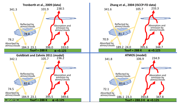
Goldblatt C, Zahnle KJ (2011) Clouds and the Faint Young Sun Paradox. Clim Past 7: 203–220. doi: 10.5194/cp-7-203-2011
![]() |
[22] | Boucher O, Randall D, Artaxo P, et al. (2013) Climate Change 2013: ThePhysical Science Basis. Contribution of Working Group I to the Fifth AssessmentReport of the Intergovernmental Panel on Climate Change. Cambridge: Cambridge University Press. |
[23] |
Rossow WB, Schiffer RA (1999) Advances in Understanding Clouds from ISCCP. Bull of the Am Meteorol Soc 80: 2261–2288. doi: 10.1175/1520-0477(1999)080<2261:AIUCFI>2.0.CO;2
![]() |
[24] |
Rossow WB, Zhang Y, Wang J (2005) A Statistical Model of Cloud Vertical Structure Based on Reconciling Cloud Layer Amounts Inferred from Satellites and Radiosonde Humidity Profiles. J Climate 18: 3587–605. doi: 10.1175/JCLI3479.1
![]() |
[25] | Laurent C, Brogniez G, Doutriaux-Boucher M, et al. (2000) Modeling of light scattering in cirrus clouds with inhomogeneous hexagonal monocrystals. Comparison with in-situ and ADEOS-POLDER measurements. Geophys Res Lett 27: 113–116. |
[26] | Yang P, Gaob BC, Baumc BA, et al. (2001) Radiative properties of cirrus clouds in the infrared (8–13µm ) spectral region. J of Quant Spectrosc & Radiat Transf 70: 473–504. |
[27] |
Yang P, Wei H, Huang HL, et al. (2005) Scattering and absorption property database for nonspherical ice particles in the near- through far-infrared spectral region. App Opt 44: 5512–5523. doi: 10.1364/AO.44.005512
![]() |
[28] |
Yang P, Bi L, Baum BA, et al. (2013) Spectrally Consistent Scattering, Absorption, and Polarization Properties of Atmospheric Ice Crystals at Wavelengths from 0.2 to 100 μm. J of the Atmos Sci 70: 330–347. doi: 10.1175/JAS-D-12-039.1
![]() |
[29] | Baum BA, Yang P, Heymsfield AJ, et al. (2005) Bulk Scattering Properties for the Remote Sensing of Ice Clouds. Part II: Narrowband Models. J of Appl Meteorol 44: 1896–1911. |
[30] |
Baum BA, Yang P, Heymsfield AJ, et al. (2011) Improvements in Shortwave Bulk Scattering and Absorption Models for the Remote Sensing of Ice Clouds. J of Appl Meteorol and Clim 50: 1037–1056. doi: 10.1175/2010JAMC2608.1
![]() |
[31] |
Baran AJ, Labonnote LC (2007) A self-consistent scattering model for cirrus. I: The solar region. Q J of the R Meteorol Soc 133: 1899–1912. doi: 10.1002/qj.164
![]() |
[32] |
Baran AJ, Connolly PJ, Lee C (2009) Testing an ensemble model of cirrus ice crystals using midlatitude in situ estimates of ice water content, volume extinction coefficient and the total solar optical depth. J of Quant Spectrosc and Radiat Trans 110: 1579–1598. doi: 10.1016/j.jqsrt.2009.02.021
![]() |
[33] |
Baran AJ (2012) From the single-scattering properties of ice crystals to climate prediction: A way forward. Atmos Res 112: 45–69. doi: 10.1016/j.atmosres.2012.04.010
![]() |
[34] | Baran AJ, Cotton R, Furtado K, et al. (2014) A self-consistent scattering model for cirrus. II: The high and low frequencies. Q J of the R Meteorol Soc 140: 1039–1057. |
[35] |
Field PR, Heymsfield AJ, Bansemer A (2007) Snow Size Distribution Parameterization for Midlatitude and Tropical Ice Clouds. J of the Atmos Sci 64: 4346–4365. doi: 10.1175/2007JAS2344.1
![]() |
[36] | Sourdeval O, Laurent C, Baran AJ, et al. (2016) A methodology for simultaneous retrieval of ice and liquid water cloud properties. Part 2: Near-global retrievals and evaluation against A-Train products. Q J of the R Meteorol Soc 142: 3063–3081. |
[37] |
Hogan RJ, Illingworth AJ (2000) Deriving cloud overlap statistics from radar. Q J of the R Meteorol Soc 126: 2903–2909. doi: 10.1002/qj.49712656914
![]() |
[38] |
Toon OB, McKay CP, Ackerman TP, et al. (1989) Rapid calculation of radiative heating rates and photodissociation rates in inhomogeneous multiple scattering atmospheres. J of Geophys Res: Atmos 94: 16287–16301. doi: 10.1029/JD094iD13p16287
![]() |
[39] |
Trenberth KE, Fasullo JT, Kiehl J (2009) Earth's Global Energy Budget. Bull of the Am Meteorol Soc 90: 311–324. doi: 10.1175/2008BAMS2634.1
![]() |
[40] | Zhang Y, Rossow WB, Lacis AA, et al. (2004) Calculation of radiative fluxes from the surface to top of atmosphere based on ISCCP and other global data sets: Refinements of the radiative transfer model and the input data. J of Geophys Res: Atmos 109. |
1. | Boris Andreianov, Abraham Sylla, Finite volume approximation and well-posedness of conservation laws with moving interfaces under abstract coupling conditions, 2023, 30, 1021-9722, 10.1007/s00030-023-00857-9 |