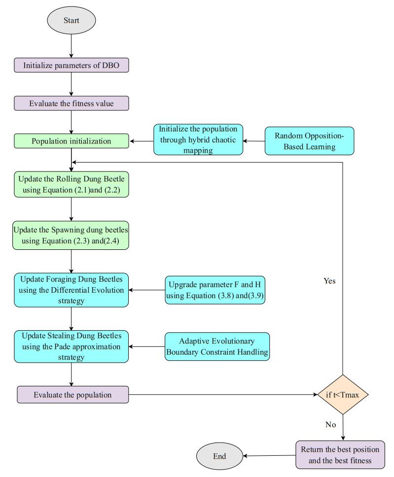
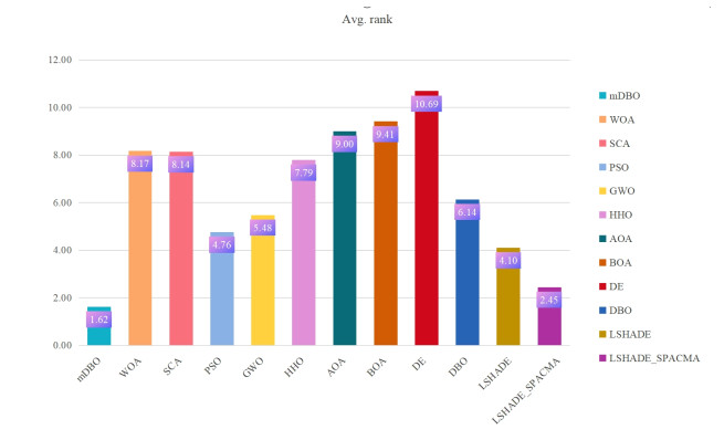
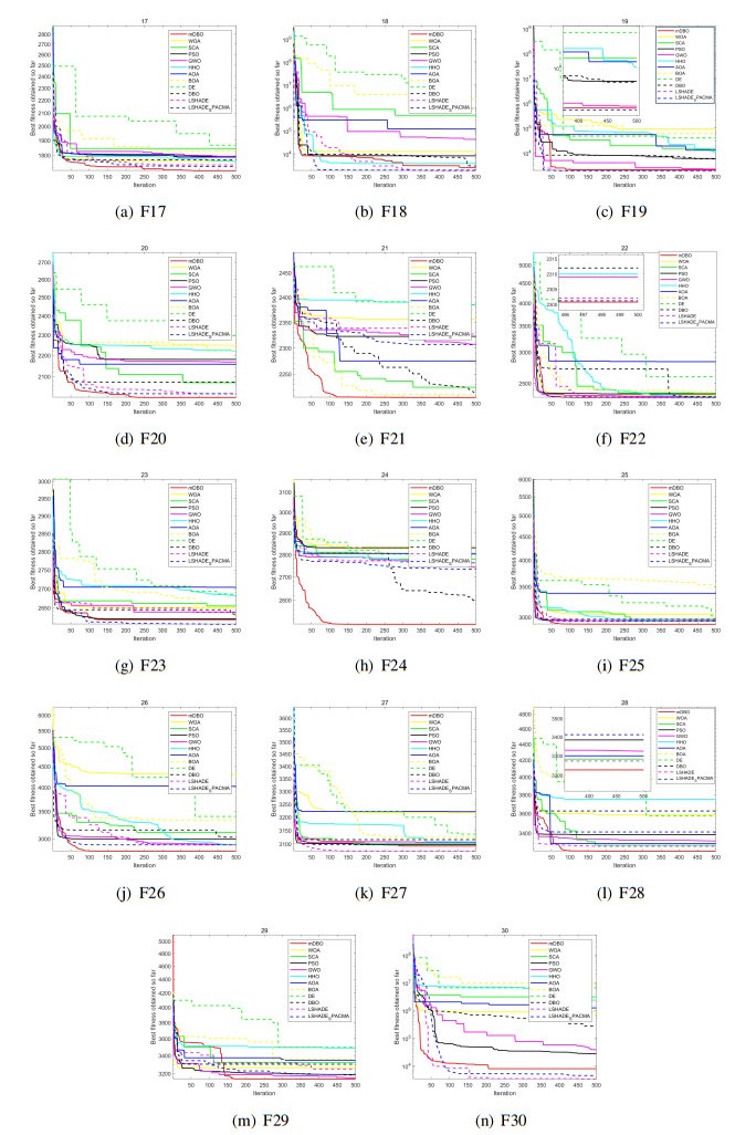
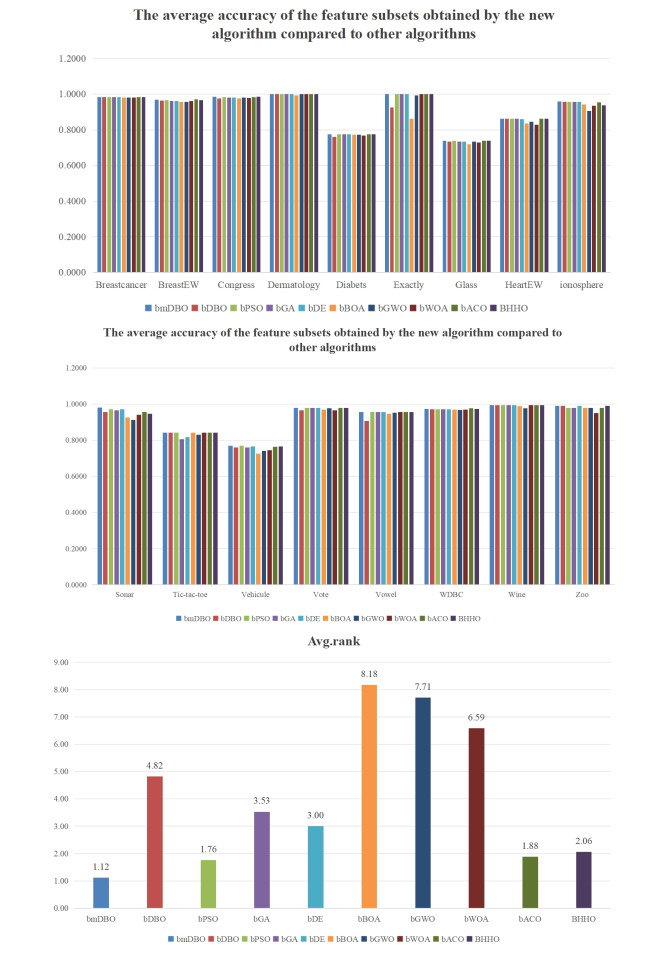
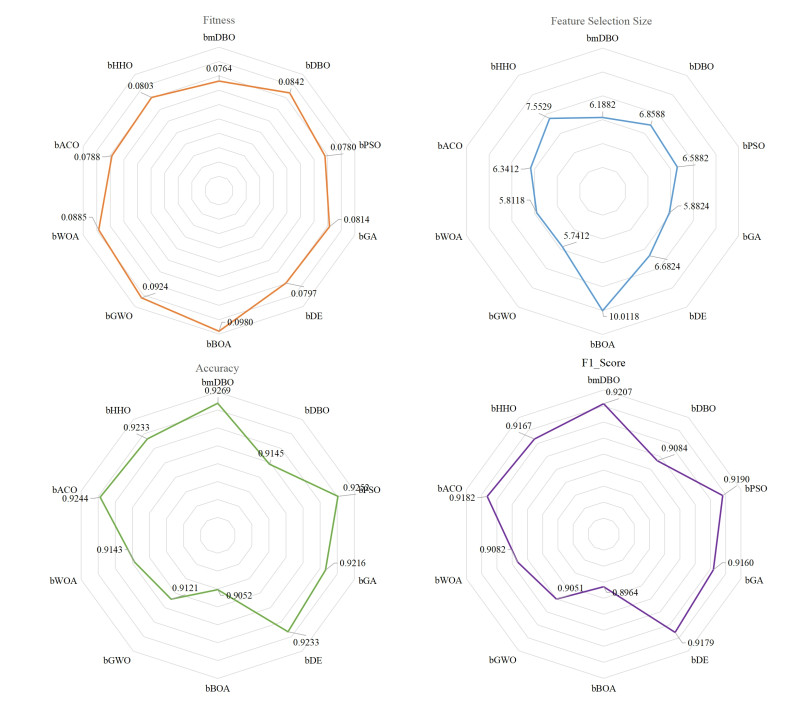
Feature selection is a crucial data processing method used to reduce dataset dimensionality while preserving key information. In this paper, we proposed a multi-strategy enhanced dung beetle optimization algorithm (mDBO) that integrates multiple strategies to effectively address the feature selection problem. First, a novel population initialization strategy based on a hybrid tent-sine map and random opposition-based learning was proposed to generate initial population. This strategy yielded a more uniform distribution of the initial population, significantly improving the quality of the population distribution within the search space. Second, a new differential evolution mutation strategy with a periodic retrospective adaptive mutation factor was proposed. This strategy effectively improved the algorithm's ability to jump out of the local optimal and explore potential candidate solutions. Third, based on Padé approximation technology and the novel adaptive evolutionary boundary constraint method, an innovative approximation strategy was proposed. The strategy was integrated into the framework of the dung beetle optimizer, significantly improving the solution accuracy and population quality of the algorithm. Finally, the binary version of the mDBO algorithm (bmDBO) was applied to feature selection tasks. Experiments entailing CEC2017 benchmark functions and 17 datasets showed that both mDBO and bmDBO outperformed other algorithms. The mDBO method outperformed other algorithms in 11 of the 29 benchmark functions, ranked second in 8 functions, and achieved an average rank of 1.62 in the Friedman ranking, securing the overall first place; the bmDBO method outperformed in 12 of 17 datasets, achieving an average ranking of 1.35 in the Friedman ranking, securing the first position.
Citation: Tianbao Liu, Lingling Yang, Yue Li, Xiwen Qin. An improved dung beetle optimizer based on Padé approximation strategy for global optimization and feature selection[J]. Electronic Research Archive, 2025, 33(3): 1693-1762. doi: 10.3934/era.2025079
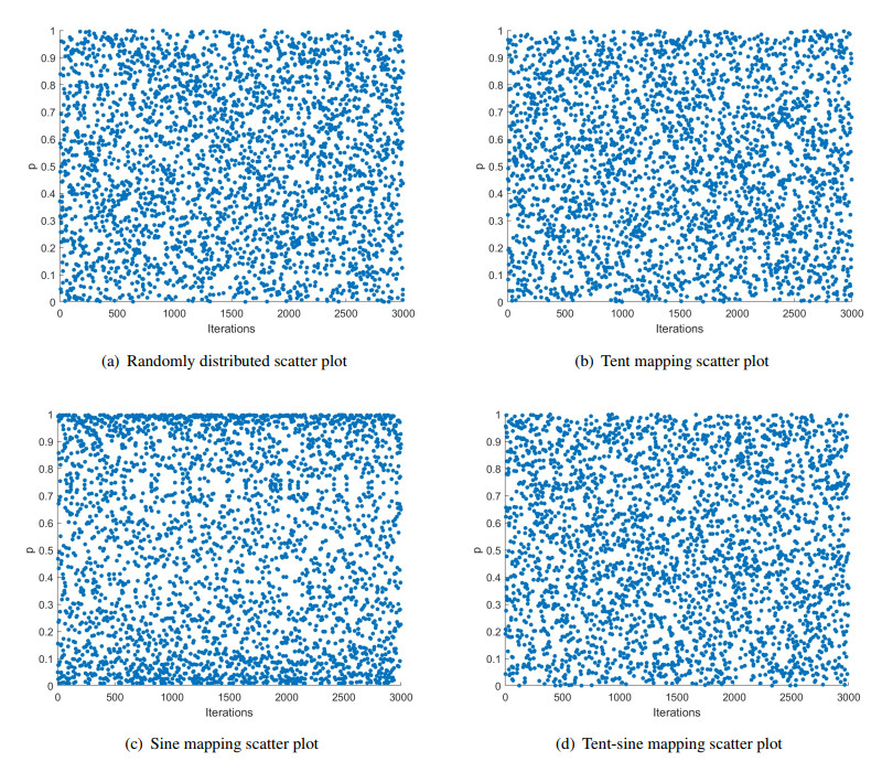
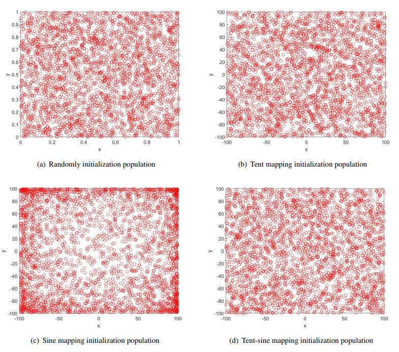
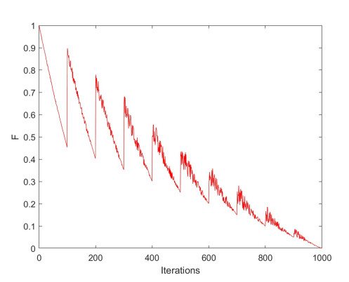
Feature selection is a crucial data processing method used to reduce dataset dimensionality while preserving key information. In this paper, we proposed a multi-strategy enhanced dung beetle optimization algorithm (mDBO) that integrates multiple strategies to effectively address the feature selection problem. First, a novel population initialization strategy based on a hybrid tent-sine map and random opposition-based learning was proposed to generate initial population. This strategy yielded a more uniform distribution of the initial population, significantly improving the quality of the population distribution within the search space. Second, a new differential evolution mutation strategy with a periodic retrospective adaptive mutation factor was proposed. This strategy effectively improved the algorithm's ability to jump out of the local optimal and explore potential candidate solutions. Third, based on Padé approximation technology and the novel adaptive evolutionary boundary constraint method, an innovative approximation strategy was proposed. The strategy was integrated into the framework of the dung beetle optimizer, significantly improving the solution accuracy and population quality of the algorithm. Finally, the binary version of the mDBO algorithm (bmDBO) was applied to feature selection tasks. Experiments entailing CEC2017 benchmark functions and 17 datasets showed that both mDBO and bmDBO outperformed other algorithms. The mDBO method outperformed other algorithms in 11 of the 29 benchmark functions, ranked second in 8 functions, and achieved an average rank of 1.62 in the Friedman ranking, securing the overall first place; the bmDBO method outperformed in 12 of 17 datasets, achieving an average ranking of 1.35 in the Friedman ranking, securing the first position.

| [1] |
M. Azizi, U. Aickelin, H. A. Khorshidi, M. Baghalzadeh-Shishehgarkhaneh, Energy valley optimizer: A novel metaheuristic algorithm for global and engineering optimization, Sci. Rep., 13 (2023), 226. https://doi.org/10.1038/s41598-022-27344-y doi: 10.1038/s41598-022-27344-y

|
| [2] |
F. A. Hashim, E. H. Houssein, K. Hussain, M. S. Mabrouk, W. Al-Atabany, Honey badger algorithm: New metaheuristic algorithm for solving optimization problems, Math. Comput. Simul., 192 (2022), 84–110. https://doi.org/10.1016/j.matcom.2021.08.013 doi: 10.1016/j.matcom.2021.08.013
|
| [3] |
S. Gupta, H. Abderazek, B. S. Yıldız, A. R. Yildiz, S. Mirjalili, S. M. Sait, Comparison of metaheuristic optimization algorithms for solving constrained mechanical design optimization problems, Exp. Syst. Appl., 183 (2021), 115351. https://doi.org/10.1016/j.eswa.2021.115351 doi: 10.1016/j.eswa.2021.115351
|
| [4] |
S. Aslan, T. Erkin, An immune plasma algorithm based approach for ucav path planning, J. King Saud Univ. Comput. Inf. Sci., 35 (2023), 56–69. https://doi.org/10.1016/j.jksuci.2022.06.004 doi: 10.1016/j.jksuci.2022.06.004
|
| [5] |
L. Abualigah, K. H. Almotairi, M. A. Elaziz, Multilevel thresholding image segmentation using meta-heuristic optimization algorithms: Comparative analysis, open challenges and new trends, Appl. Intell., 53 (2023), 11654–11704. https://doi.org/10.1007/s10489-022-04064-4 doi: 10.1007/s10489-022-04064-4
|
| [6] |
M. Chan-Ley, G. Olague, Categorization of digitized artworks by media with brain programming, Appl. Opt., 59 (2020), 4437–4447, 2020. https://doi.org/10.1364/AO.385552 doi: 10.1364/AO.385552
|
| [7] |
Y. Li, G. Tian, Y. Yi, Y. Yuan, Improved artificial rabbit optimization and its application in multichannel signal denoising, IEEE Sensors J., 2024 (2024). https://doi.org/10.1109/JSEN.2024.3456290 doi: 10.1109/JSEN.2024.3456290
|
| [8] |
Y. Xiao, H. Cui, A. G. Hussien, F. A. Hashim, MSAO: A multi-strategy boosted snow ablation optimizer for global optimization and real-world engineering applications, Adv. Eng. Inf., 61 (2024), 102464. https://doi.org/10.1016/j.aei.2024.102464 doi: 10.1016/j.aei.2024.102464
|
| [9] |
X. Fei, J. Wang, S. Ying, Z. Hu, J. Shi, Projective parameter transfer based sparse multiple empirical kernel learning machine for diagnosis of brain disease, Neurocomputing, 413 (2020), 271–283. https://doi.org/10.1016/j.neucom.2020.07.008 doi: 10.1016/j.neucom.2020.07.008
|
| [10] |
Z. Ma, X. Li, An improved supervised and attention mechanism-based u-net algorithm for retinal vessel segmentation, Comput. Biol. Med., 168 (2024), 107770. https://doi.org/10.1016/j.compbiomed.2023.107770 doi: 10.1016/j.compbiomed.2023.107770
|
| [11] |
Y. Xiao, Y. Guo, H. Cui, Y. Wang, J. Li, Y. Zhang, IHAOAVOA: An improved hybrid aquila optimizer and African vultures optimization algorithm for global optimization problems, Math. Biosci. Eng., 19 (2022), 10963–11017. https://doi.org/10.3934/mbe.2022512 doi: 10.3934/mbe.2022512
|
| [12] |
J. Zhang, M. Xiao, L. Gao, Q. Pan, Queuing search algorithm: A novel metaheuristic algorithm for solving engineering optimization problems, Appl. Math. Modell., 63 (2018), 464–490. https://doi.org/10.1016/j.apm.2018.06.036 doi: 10.1016/j.apm.2018.06.036
|
| [13] |
U. Kamath, K. De Jong, A. Shehu, Effective automated feature construction and selection for classification of biological sequences, PloS One, 9 (2014), e99982. https://doi.org/10.1371/journal.pone.0099982 doi: 10.1371/journal.pone.0099982
|
| [14] |
F. Thabtah, F. Kamalov, S. Hammoud, S. R. Shahamiri, Least loss: A simplified filter method for feature selection, Inf. Sci., 534 (2020), 1–15. https://doi.org/10.1016/j.ins.2020.05.017 doi: 10.1016/j.ins.2020.05.017
|
| [15] |
L. Sun, J. Zhang, W. Ding, J. Xu, Feature reduction for imbalanced data classification using similarity-based feature clustering with adaptive weighted k-nearest neighbors, Inf. Sci., 593 (2022), 591–613. https://doi.org/10.1016/j.ins.2022.02.004 doi: 10.1016/j.ins.2022.02.004
|
| [16] |
Z. Tao, L. Huiling, W. Wenwen, Y. Xia, GA-SVM based feature selection and parameter optimization in hospitalization expense modeling, Appl. Soft Comput., 75 (2019), 323–332. https://doi.org/10.1016/j.asoc.2018.11.001 doi: 10.1016/j.asoc.2018.11.001
|
| [17] | H. Liu, Z. Zhao, Manipulating data and dimension reduction methods: Feature selection, in Computational Complexity: Theory, Techniques, and Applications, Springer, (2012), 790–1800. https://doi.org/10.1007/978-1-4614-1800-9_115 |
| [18] |
M. Rostami, K. Berahmand, E. Nasiri, S. Forouzandeh, Review of swarm intelligence-based feature selection methods, Eng. Appl. Artif. Intell., 100 (2021), 104210. https://doi.org/10.1016/j.engappai.2021.104210 doi: 10.1016/j.engappai.2021.104210
|
| [19] |
D. H. Wolpert, W. G. Macready, No free lunch theorems for optimization, IEEE Trans. Evol. Comput., 1 (1997), 67–82. https://doi.org/10.1109/4235.585893 doi: 10.1109/4235.585893
|
| [20] |
X. Song, Y. Zhang, D. Gong, X. Sun, Feature selection using bare-bones particle swarm optimization with mutual information, Pattern Recognit., 112 (2021), 107804. https://doi.org/10.1016/j.patcog.2020.107804 doi: 10.1016/j.patcog.2020.107804
|
| [21] |
H. Faris, M. M. Mafarja, A. A. Heidari, I. Aljarah, A. M. Al-Zoubi, S. Mirjalili, et al., An efficient binary salp swarm algorithm with crossover scheme for feature selection problems, Knowl. Based Syst., 154 (2018), 43–67. https://doi.org/10.1016/j.knosys.2018.05.009 doi: 10.1016/j.knosys.2018.05.009
|
| [22] |
E. Emary, H. M. Zawbaa, A. E. Hassanien, Binary grey wolf optimization approaches for feature selection, Neurocomputing, 172 (2016), 371–381. https://doi.org/10.1016/j.neucom.2015.06.083 doi: 10.1016/j.neucom.2015.06.083
|
| [23] |
Y. Zhao, J. Dong, X. Li, H. Chen, S. Li, A binary dandelion algorithm using seeding and chaos population strategies for feature selection, Appl. Soft Comput., 125 (2022), 109166. https://doi.org/10.1016/j.asoc.2022.109166 doi: 10.1016/j.asoc.2022.109166
|
| [24] |
M. Mafarja, S. Mirjalili, Whale optimization approaches for wrapper feature selection, Appl. Soft Comput., 62 (2018), 441–453. https://doi.org/10.1016/j.asoc.2017.11.006 doi: 10.1016/j.asoc.2017.11.006
|
| [25] |
A. Adamu, M. Abdullahi, S. B. Junaidu, I. H. Hassan, An hybrid particle swarm optimization with crow search algorithm for feature selection, Mach. Learn. Appl., 6 (2021), 100108. https://doi.org/10.1016/j.mlwa.2021.100108 doi: 10.1016/j.mlwa.2021.100108
|
| [26] |
Y. Xue, T. Tang, A. X. Liu, Large-scale feedforward neural network optimization by a self-adaptive strategy and parameter based particle swarm optimization, IEEE Access, 7 (2019), 52473–52483. https://doi.org/10.1109/ACCESS.2019.2911530 doi: 10.1109/ACCESS.2019.2911530
|
| [27] |
E. Aličković, A. Subasi, Breast cancer diagnosis using GA feature selection and rotation forest, Neural Comput. Appl., 28 (2017), 753–763. https://doi.org/10.1007/s00521-015-2103-9 doi: 10.1007/s00521-015-2103-9
|
| [28] |
B. Xue, M. Zhang, W. N. Browne, X. Yao, A survey on evolutionary computation approaches to feature selection, IEEE Trans. Evol. Comput., 20 (2015), 606–626. https://doi.org/10.1109/TEVC.2015.2504420 doi: 10.1109/TEVC.2015.2504420
|
| [29] |
N. Khodadadi, E. Khodadadi, Q. Al-Tashi, E. S. M. El-Kenawy, L. Abualigah, S. J. Abdulkadir, et al., BAOA: Binary arithmetic optimization algorithm with K-nearest neighbor classifier for feature selection, IEEE Access, 11 (2023), 94094–94115. https://doi.org/10.1109/ACCESS.2023.3310429 doi: 10.1109/ACCESS.2023.3310429
|
| [30] |
W. N. Chen, D. Z. Tan, Q. Yang, T. Gu, J. Zhang, Ant colony optimization for the control of pollutant spreading on social networks, IEEE Trans. Cybern., 50 (2019), 4053–4065. https://doi.org/10.1109/TCYB.2019.2922266 doi: 10.1109/TCYB.2019.2922266
|
| [31] |
H. Hichem, M. Elkamel, M. Rafik, M. T. Mesaaoud, C. Ouahiba, A new binary grasshopper optimization algorithm for feature selection problem, J. King Saud University Comput. Inf. Sci., 34 (2022), 316–328. https://doi.org/10.1016/j.jksuci.2019.11.007 doi: 10.1016/j.jksuci.2019.11.007
|
| [32] |
A. A. Alhussan, A. A. Abdelhamid, E. S. M. El-Kenawy, A. Ibrahim, M. M. Eid, D. S. Khafaga, et al., A binary waterwheel plant optimization algorithm for feature selection, IEEE Access, 11 (2023), 94227–94251. https://doi.org/10.1109/ACCESS.2023.3312022 doi: 10.1109/ACCESS.2023.3312022
|
| [33] |
K. Nag, N. R. Pal, A multiobjective genetic programming-based ensemble for simultaneous feature selection and classification, IEEE Trans. Cybern., 46 (2015), 499–510. https://doi.org/10.1109/TCYB.2015.2404806 doi: 10.1109/TCYB.2015.2404806
|
| [34] |
J. Xue, B. Shen, Dung beetle optimizer: A new meta-heuristic algorithm for global optimization, J. Supercomput., 79 (2023), 7305–7336. https://doi.org/10.1007/s11227-022-04959-6 doi: 10.1007/s11227-022-04959-6
|
| [35] |
X. Yao, Y. Liu, G. Lin, Evolutionary programming made faster, IEEE Trans. Evol. Comput., 3 (1999), 82–102. https://doi.org/10.1109/4235.771163 doi: 10.1109/4235.771163
|
| [36] |
T. Y. Wu, H. Li, S. C. Chu, CPPE: An improved phasmatodea population evolution algorithm with chaotic maps, Mathematics, 11 (2023), 1977. https://doi.org/10.3390/math11091977 doi: 10.3390/math11091977
|
| [37] |
P. Qu, Q. Yuan, F. Du, Q. Gao, An improved manta ray foraging optimization algorithm, Sci. Rep., 14 (2024), 10301. https://doi.org/10.1038/s41598-024-59960-1 doi: 10.1038/s41598-024-59960-1
|
| [38] |
H. Yu, Y. Wang, H. Jia, L. Abualigah, Modified prairie dog optimization algorithm for global optimization and constrained engineering problems, Math. Biosci. Eng, 20 (2023), 19086–19132. https://doi.org/10.3934/mbe.2023844 doi: 10.3934/mbe.2023844
|
| [39] |
C. Liu, L. Li, Y. Qiang, S. Zhang, Predicting construction accidents on sites: An improved atomic search optimization algorithm approach, Eng. Rep., 6 (2024), e12773. https://doi.org/10.1002/eng2.12773 doi: 10.1002/eng2.12773
|
| [40] |
A. Bisht, M. Dua, S. Dua, A novel approach to encrypt multiple images using multiple chaotic maps and chaotic discrete fractional random transform, J. Ambient Intell. Humanized Comput., 10 (2019), 3519–3531. https://doi.org/10.1007/s12652-018-1072-0 doi: 10.1007/s12652-018-1072-0
|
| [41] |
Y. Zhou, L. Bao, C. L. P. Chen, A new 1D chaotic system for image encryption, Signal Process., 97 (2014), 172–182. https://doi.org/10.1016/j.sigpro.2013.10.034 doi: 10.1016/j.sigpro.2013.10.034
|
| [42] |
F. Han, X. Liao, B. Yang, Y. Zhang, A hybrid scheme for self-adaptive double color-image encryption, Multimedia Tools Appl., 77 (2018), 14285–14304. https://doi.org/10.1007/s11042-017-5029-7 doi: 10.1007/s11042-017-5029-7
|
| [43] | H. R. Tizhoosh, Opposition-based learning: A new scheme for machine intelligence, in International Conference on Computational Intelligence for Modelling, Control and Automation and International Conference on Intelligent Agents, Web Technologies and Internet Commerce (CIMCA-IAWTIC'06), 1 (2005), 695–701. https://doi.org/10.1109/CIMCA.2005.1631345 |
| [44] |
S. Rahnamayan, H. R. Tizhoosh, M. M. A. Salama, Opposition-based differential evolution, IEEE Trans. Evol. Comput., 12 (2008), 64–79. https://doi.org/10.1109/TEVC.2007.894200 doi: 10.1109/TEVC.2007.894200
|
| [45] |
H. Wang, Z. Wu, S. Rahnamayan, Y. Liu, M. Ventresca, Enhancing particle swarm optimization using generalized opposition-based learning, Inf. Sci., 181 (2011), 4699–4714. https://doi.org/10.1016/j.ins.2011.03.016 doi: 10.1016/j.ins.2011.03.016
|
| [46] |
M. Abd Elaziz, D. Oliva, S. Xiong, An improved opposition-based sine cosine algorithm for global optimization, Exp. Syst. Appl., 90 (2017), 484–500. https://doi.org/10.1016/j.eswa.2017.07.043 doi: 10.1016/j.eswa.2017.07.043
|
| [47] |
W. Long, J. Jiao, X. Liang, S. Cai, M. Xu, A random opposition-based learning grey wolf optimizer, IEEE Access, 7 (2019), 113810–113825. https://doi.org/10.1109/ACCESS.2019.2934994 doi: 10.1109/ACCESS.2019.2934994
|
| [48] |
R. Storn, K. Price, Differential evolution–-a simple and efficient heuristic for global optimization over continuous spaces, J. Global Optim., 11 (1997), 341–359. https://doi.org/10.1023/A:1008202821328 doi: 10.1023/A:1008202821328
|
| [49] |
A. Nickabadi, M. M. Ebadzadeh, R. Safabakhsh, A novel particle swarm optimization algorithm with adaptive inertia weight, Appl. Soft Comput., 11 (2011), 3658–3670. https://doi.org/10.1016/j.asoc.2011.01.037 doi: 10.1016/j.asoc.2011.01.037
|
| [50] |
Y. Honshuku, H. Isakari, A topology optimisation of acoustic devices based on the frequency response estimation with the Padé approximation, Appl. Math. Modell., 110 (2022), 819–840. https://doi.org/10.1016/j.apm.2022.06.020 doi: 10.1016/j.apm.2022.06.020
|
| [51] |
H. Vazquez-Leal, B. Benhammouda, U. Filobello-Nino, A. Sarmiento-Reyes, V. M. Jimenez-Fernandez, J. L. Garcia-Gervacio, et al., Direct application of Padé approximant for solving nonlinear differential equations, SpringerPlus, 3 (2014), 1–11. https://doi.org/10.1186/2193-1801-3-563 doi: 10.1186/2193-1801-3-563
|
| [52] |
I. V. Andrianov, A. Shatrov, Padé approximants, their properties, and applications to hydrodynamic problems, Symmetry, 13 (2021), 1869. https://doi.org/10.3390/sym13101869 doi: 10.3390/sym13101869
|
| [53] |
J. Xu, T. Wang, L. Pei, S. Mao, C. Zhu, Parameter identification of electrolyte decomposition state in lithium-ion batteries based on a reduced pseudo two-dimensional model with Padé approximation, J. Power Sources, 460 (2020), 228093. https://doi.org/10.1016/j.jpowsour.2020.228093 doi: 10.1016/j.jpowsour.2020.228093
|
| [54] |
A. H. Gandomi, X. S. Yang, Evolutionary boundary constraint handling scheme, Neural Comput. Appl., 21 (2012), 1449–1462. https://doi.org/10.1007/s00521-012-1069-0 doi: 10.1007/s00521-012-1069-0
|
| [55] | A. H. Gandomi, A. R. Kashani, Evolutionary bound constraint handling for particle swarm optimization, in 2016 4th International Symposium on Computational and Business Intelligence (ISCBI), (2016), 148–152. https://doi.org/10.1109/ISCBI.2016.7743274 |
| [56] | A. H. Gandomi, A. R. Kashani, M. Mousavi, Boundary constraint handling affection on slope stability analysis, in Engineering and Applied Sciences Optimization. Computational Methods in Applied Sciences (eds. N. Lagaros and M. Papadrakakis), Springer, (2015), 341–358. https://doi.org/10.1007/978-3-319-18320-6_18 |
| [57] |
A. H. Gandomi, A. R. Kashani, F. Zeighami, Retaining wall optimization using interior search algorithm with different bound constraint handling, Int. J. Numer. Anal. Methods Geomech., 41 (2017), 1304–1331. https://doi.org/10.1002/nag.2678 doi: 10.1002/nag.2678
|
| [58] |
A. C. Cinar, A comprehensive comparison of accuracy-based fitness functions of metaheuristics for feature selection, Soft Comput., 27 (2023), 8931–8958. https://doi.org/10.1007/s00500-023-08414-3 doi: 10.1007/s00500-023-08414-3
|
| [59] |
I. Al-Shourbaji, N. Helian, Y. Sun, S. Alshathri, M. Abd Elaziz, Boosting ant colony optimization with reptile search algorithm for churn prediction, Mathematics, 10 (2022), 1031. https://doi.org/10.3390/math10071031 doi: 10.3390/math10071031
|
| [60] | E. S. M. El-Kenawy, S. Mirjalili, A. Ibrahim, M. Alrahmawy, M. El-Said, R. M. Zaki, et al., Advanced meta-heuristics, convolutional neural networks, and feature selectors for efficient COVID-19 X-ray chest image classification, IEEE Access, 9 (2021). 36019–36037. https://doi.org/10.1109/ACCESS.2021.3061058 |
| [61] | T. Khosla, O. P. Verma, An adaptive hybrid particle swarm optimizer for constrained optimization problem, in 2021 International Conference in Advances in Power, Signal, and Information Technology (APSIT), IEEE, (2021), 1–7. https://doi.org/10.1109/APSIT52773.2021.9641410 |
| [62] |
B. D. Kwakye, Y. Li, H. H. Mohamed, E. Baidoo, T. Q. Asenso, Particle guided metaheuristic algorithm for global optimization and feature selection problem, Exp. Syst. Appl., 248 (2024), 123362. https://doi.org/10.1016/j.eswa.2024.123362 doi: 10.1016/j.eswa.2024.123362
|
| [63] | G. Wu, R. Mallipeddi, P. N. Suganthan, Problem definitions and evaluation criteria for the CEC 2017 competition on constrained real-parameter optimization, National University of Defense Technology, Changsha, Hunan, PR China and Kyungpook National University, Daegu, South Korea and Nanyang Technological University, Singapore, Technical Report, 2017. |
| [64] |
S. Mirjalili, A. Lewis, The whale optimization algorithm, Adv. Eng. Software, 95 (2016), 51–67. https://doi.org/10.1016/j.advengsoft.2016.01.008 doi: 10.1016/j.advengsoft.2016.01.008
|
| [65] |
S. Mirjalili, SCA: A sine cosine algorithm for solving optimization problems, Knowl. Based Syst., 96 (2016), 120–133. https://doi.org/10.1016/j.knosys.2015.12.022 doi: 10.1016/j.knosys.2015.12.022
|
| [66] | J. Kennedy, R. Eberhart, Particle swarm optimization, in Proceedings of ICNN'95-International Conference on Neural Networks, 4 (1995), 1942–1948. https://doi.org/10.1109/ICNN.1995.488968 |
| [67] |
S. Mirjalili, S. M. Mirjalili, A. Lewis, Grey wolf optimizer, Adv. Eng. Software, 69 (2014), 46–61. https://doi.org/10.1016/j.advengsoft.2013.12.007 doi: 10.1016/j.advengsoft.2013.12.007
|
| [68] |
A. A. Heidari, S. Mirjalili, H. Faris, I. Aljarah, M. Mafarja, H. Chen, Harris Hawks optimization: Algorithm and applications, Future Gener. Comput. Syst., 97 (2019), 849–872. https://doi.org/10.1016/j.future.2019.02.028 doi: 10.1016/j.future.2019.02.028
|
| [69] |
L. Abualigah, A. Diabat, S. Mirjalili, M Abd Elaziz, A. H. Gandomi, The arithmetic optimization algorithm, Comput. Methods Appl. Mech. Eng., 376 (2021), 113609. https://doi.org/10.1016/j.cma.2020.113609 doi: 10.1016/j.cma.2020.113609
|
| [70] |
S. Arora, P. Anand, Binary butterfly optimization approaches for feature selection, Exp. Syst. Appl., 116 (2019), 147–160. https://doi.org/10.1016/j.eswa.2018.08.051 doi: 10.1016/j.eswa.2018.08.051
|
| [71] | R. Tanabe, A. S. Fukunaga, Improving the search performance of SHADE using linear population size reduction, in 2014 IEEE Congress on Evolutionary Computation (CEC), (2014), 1658–1665. https://doi.org/10.1109/CEC.2014.6900380 |
| [72] | A. W. Mohamed, A. A. Hadi, A. M. Fattouh, K. M. Jambi, LSHADE with semi-parameter adaptation hybrid with CMA-ES for solving CEC 2017 benchmark problems, in 2017 IEEE Congress on Evolutionary Computation (CEC), (2017), 145–152. https://doi.org/10.1109/CEC.2017.7969307 |
| [73] |
S. Zhao, Y. Wu, S. Tan, J. Wu, Z. Cui, Y. G. Wang, QQLMPA: A quasi-opposition learning and Q-learning based marine predators algorithm, Exp. Syst. Appl., 213 (2023), 119246. https://doi.org/10.1016/j.eswa.2022.119246 doi: 10.1016/j.eswa.2022.119246
|
| [74] |
Y. Xu, Z. Yang, X. Li, H. Kang, X. Yang, Dynamic opposite learning enhanced teaching-learning-based optimization, Knowl. Based Syst., 188 (2020), 104966. https://doi.org/10.1016/j.knosys.2019.104966 doi: 10.1016/j.knosys.2019.104966
|
| [75] | R. W. Morrison, Designing Evolutionary Algorithms for Dynamic Environments, Springer, 2004. https://doi.org/10.1007/978-3-662-06560-0 |
| [76] |
K. Hussain, M. N. M. Salleh, S. Cheng, Y. Shi, On the exploration and exploitation in popular swarm-based metaheuristic algorithms, Neural Comput. Appl., 31 (2019), 7665–7683. https://doi.org/10.1007/s00521-018-3592-0 doi: 10.1007/s00521-018-3592-0
|
| [77] |
S. Cheng, Y. Shi, Q. Qin, Q. Zhang, R. Bai, Population diversity maintenance in brain storm optimization algorithm, J. Artif. Intell. Soft Comput. Res., 4 (2014), 83–97. https://doi.org/10.1515/jaiscr-2015-0001 doi: 10.1515/jaiscr-2015-0001
|
| [78] |
S. Mirjalili, A. Lewis, S-shaped versus V-shaped transfer functions for binary particle swarm optimization, Swarm Evol. Comput., 9 (2013), 1–14. https://doi.org/10.1016/j.swevo.2012.09.002 doi: 10.1016/j.swevo.2012.09.002
|
| [79] |
J. Too, A. R. Abdullah, N. Mohd-Saad, Hybrid binary particle swarm optimization differential evolution-based feature selection for emg signals classification, Axioms, 8 (2019), 79. https://doi.org/10.3390/axioms8030079 doi: 10.3390/axioms8030079
|
| [80] |
J. Too, A. R. Abdullah, N. Mohd-Saad, N. Mohd-Ali, W. Tee, A new competitive binary grey wolf optimizer to solve the feature selection problem in emg signals classification, Computers, 7 (2018), 58. https://doi.org/10.3390/computers7040058 doi: 10.3390/computers7040058
|
| [81] |
M. H. Aghdam, N. Ghasem-Aghaee, M. E. Basiri, Text feature selection using ant colony optimization, Exp. Syst. Appl., 36 (2009), 6843–6853. https://doi.org/10.1016/j.eswa.2008.08.022 doi: 10.1016/j.eswa.2008.08.022
|
| [82] |
J. Too, A. R. Abdullah, N. Mohd-Saad, A new quadratic binary harris hawk optimization for feature selection, Electronics, 8 (2019), 1130. https://doi.org/10.3390/electronics8101130 doi: 10.3390/electronics8101130
|
Figures(19) / Tables(27)
Tianbao Liu, Lingling Yang, Yue Li, Xiwen Qin. An improved dung beetle optimizer based on Padé approximation strategy for global optimization and feature selection[J]. Electronic Research Archive, 2025, 33(3): 1693-1762. doi: 10.3934/era.2025079


 DownLoad: