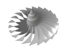
In this paper, we introduce a dimension splitting method for simulating the air flow state of the aeroengine turbine fan. Based on the geometric model of the fan blade, the dimension splitting method establishes a semi-geodesic coordinate system. Under such coordinate system, the Navier-Stokes equations are reformulated into the combination of membrane operator equations on two-dimensional manifolds and bending operator equations along the hub circle. Using Euler central difference scheme to approximate the third variable, the new form of Navier-Stokes equations is splitting into a set of two-dimensional sub-problems. Solving these sub-problems by alternate iteration, it follows an approximate solution to Navier-Stokes equations. Furthermore, we conduct a numerical experiment to show that the dimension splitting method has a good performance by comparing with the traditional methods. Finally, we give the simulation results of the pressure and flow state of the fan blade.
Citation: Guoliang Ju, Can Chen, Rongliang Chen, Jingzhi Li, Kaitai Li, Shaohui Zhang. Numerical simulation for 3D flow in flow channel of aeroengine turbine fan based on dimension splitting method[J]. Electronic Research Archive, 2020, 28(2): 837-851. doi: 10.3934/era.2020043
In this paper, we introduce a dimension splitting method for simulating the air flow state of the aeroengine turbine fan. Based on the geometric model of the fan blade, the dimension splitting method establishes a semi-geodesic coordinate system. Under such coordinate system, the Navier-Stokes equations are reformulated into the combination of membrane operator equations on two-dimensional manifolds and bending operator equations along the hub circle. Using Euler central difference scheme to approximate the third variable, the new form of Navier-Stokes equations is splitting into a set of two-dimensional sub-problems. Solving these sub-problems by alternate iteration, it follows an approximate solution to Navier-Stokes equations. Furthermore, we conduct a numerical experiment to show that the dimension splitting method has a good performance by comparing with the traditional methods. Finally, we give the simulation results of the pressure and flow state of the fan blade.

| [1] |
An introduction to differential geometry with applications to elasticity. Journal of Turbomachinery (2005) 78: 1-215. 
|
| [2] |
J. DeCastro, J. Litt and D. Frederick, A modular aero-propulsion system simulation of a large commercial aircraft engine, 44th AIAA/ASME/SAE/ASEE Joint Propulsion Conference & Exhibit, (2008), 4579. doi: 10.2514/6.2008-4579
|
| [3] |
Navier-Stokes analysis methods for turbulent jet flows with application to aircraft exhaust nozzles. Progress in Aerospace Sciences (2006) 42: 377-418.
|
| [4] |
Three-dimensional navier-stokes computations of transonic fan flow using an explicit flow solver and an implicit solver. Journal of Elasticity (1993) 115: 261-272.
|
| [5] | (2013) Navier-Stokes Boundary Shape Control, Dimension Splitting Method and its Application(in Chinese). Beijing: 1nd ed., Science Press. |
| [6] |
A novel variational method for 3D viscous flow in flow channel of turbomachines based on differential geometry. Applicable Analysis (2019) 1: 1-17.
|
| [7] |
Numerical investigation of transonic flow over deformable airfoil with plunging motion. Applied Mathematics and Mechanics (2016) 37: 75-96.
|
| [8] | (1983) Semi-Riemannian Geometry with Applications to Relativity. alt Lake: Academic press. |
| [9] | H. Schlichting and K. Gersten, Boundary-layer Theory, 9nd ed., Springer, Berlin, 2016. |
| [10] |
Computational analysis of flow-driven string dynamics in turbomachinery. Computers Fluids (2017) 142: 109-117.
|
| [11] |
Large-scale multifidelity, multiphysics, hybrid Reynolds-averaged Navier-Stokes/large-eddy simulation of an installed aeroengine. Journal of Propulsion and Power (2016) 1: 997-1008.
|
| [12] |
Aeroengine turbine blade containment tests using high-speed rotor spin testing facility. Aerospace Science and Technology (2006) 10: 501-508.
|
| [13] |
J. Yeuan, T. Liang and A. Hamed, A 3-D Navier-Stokes solver for turbomachinery blade rows, 32nd Joint Propulsion Conference and Exhibit, (1996), 3308. doi: 10.2514/6.1996-3308
|
| [14] | Numerical study on blade un-running design of a transonic fan. Journal of Mechanical Engineering (2013) 49: 147-153. |
| [15] |
Estimation of impacts of removing arbitrarily constrained domain details to the analysis of incompressible fluid flows. Communications in Computational Physics (2016) 20: 944-968.
|
| [16] |
A weak Galerkin finite element method for the Navier-Stokes equations. Communications in Computational Physics (2018) 23: 706-746.
|


Figures(16)
Guoliang Ju, Can Chen, Rongliang Chen, Jingzhi Li, Kaitai Li, Shaohui Zhang. Numerical simulation for 3D flow in flow channel of aeroengine turbine fan based on dimension splitting method[J]. Electronic Research Archive, 2020, 28(2): 837-851. doi: 10.3934/era.2020043


 DownLoad: