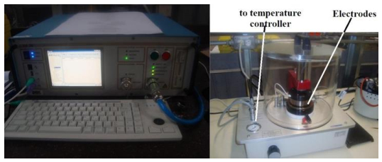
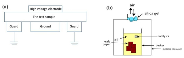
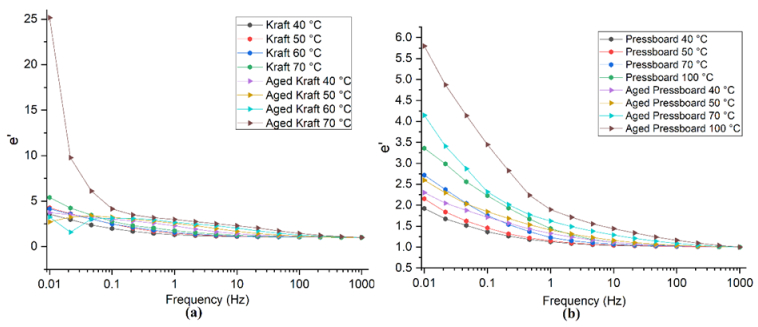
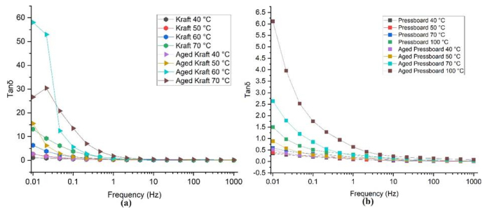
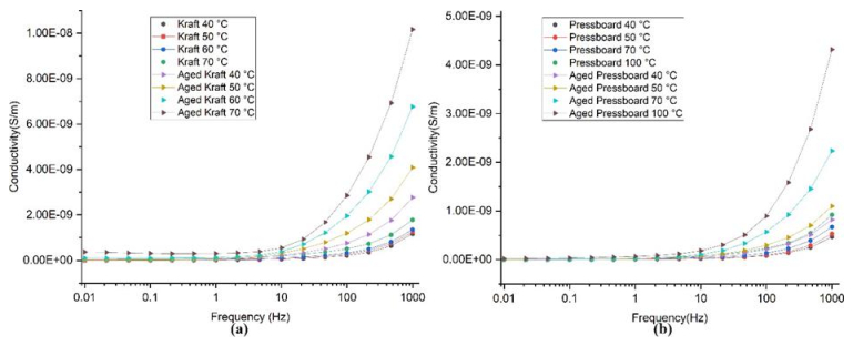
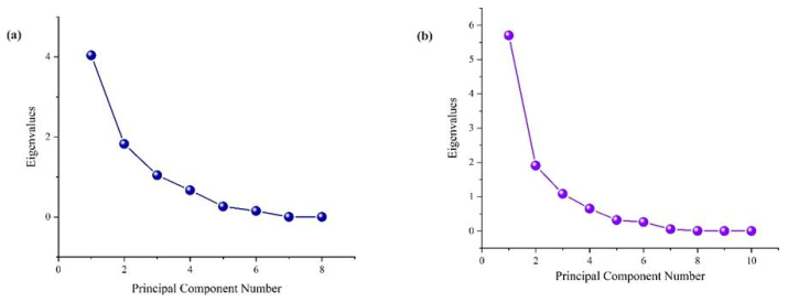
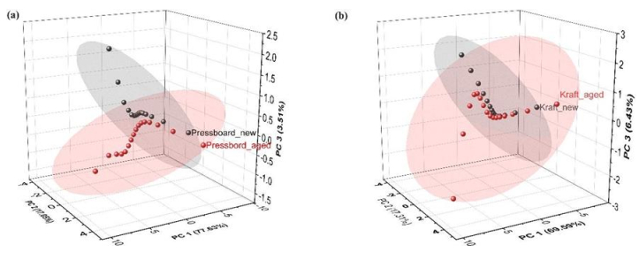
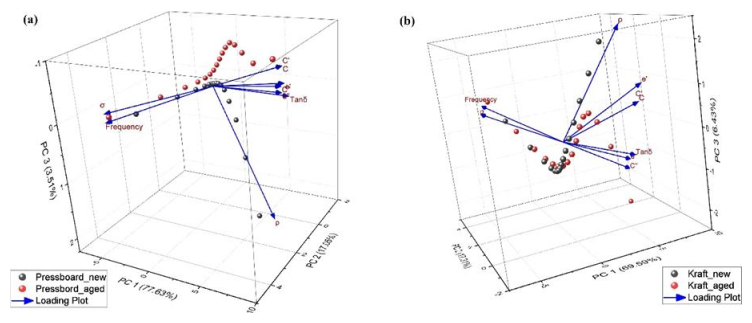
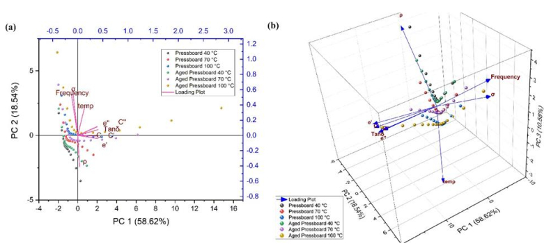
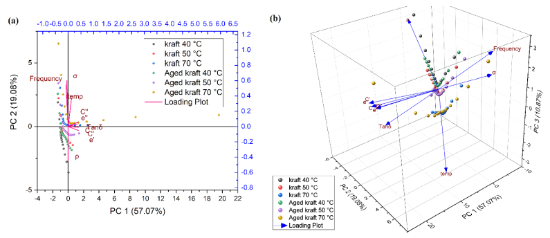
We explored the aging effects on insulating materials used in power transformers through dielectric spectroscopy. Frequency domain spectroscopy (FDS) was conducted for both aged and new Kraft paper and pressboard samples to determine their dielectric properties across a temperature range of 40–100 ℃ for pressboard and 40–70 ℃ for Kraft paper. Principal component analysis (PCA) was employed to classify the data, identify key factors contributing to variance, and elucidate the relationships between different parameters. The analysis revealed positive correlations between conductivity and frequency, as well as between permittivity and tan delta, with distinct differences in behavior observed between aged and new samples at lower frequencies. Additionally, the impact of temperature was evident, with increased temperature leading to an upward shift in dielectric behavior. At lower temperatures, aging had a reduced effect on the materials' properties. These findings provide significant insights into the dielectric behavior and aging mechanisms of insulation materials in power transformers.
Citation: Souhaib Cherrak, Tahar Seghier, Ali Benghia, Felipe Araya Machuca, Augustin Mpanda Mabwe, Souraya Goumri-Said. Exploring the electrical properties of pressboard and kraft paper insulation in power transformers: A dielectric spectroscopy and principal component analysis approach[J]. AIMS Environmental Science, 2024, 11(5): 831-846. doi: 10.3934/environsci.2024041
We explored the aging effects on insulating materials used in power transformers through dielectric spectroscopy. Frequency domain spectroscopy (FDS) was conducted for both aged and new Kraft paper and pressboard samples to determine their dielectric properties across a temperature range of 40–100 ℃ for pressboard and 40–70 ℃ for Kraft paper. Principal component analysis (PCA) was employed to classify the data, identify key factors contributing to variance, and elucidate the relationships between different parameters. The analysis revealed positive correlations between conductivity and frequency, as well as between permittivity and tan delta, with distinct differences in behavior observed between aged and new samples at lower frequencies. Additionally, the impact of temperature was evident, with increased temperature leading to an upward shift in dielectric behavior. At lower temperatures, aging had a reduced effect on the materials' properties. These findings provide significant insights into the dielectric behavior and aging mechanisms of insulation materials in power transformers.

| [1] |
Yuan Z, Wang Q, Ren Z, et al. (2023) Investigating aging characteristics of oil-immersed power transformers insulation in electrical-thermal-mechanical combined conditions. Polymers 15: 4239. https://doi.org/10.3390/polym15214239 doi: 10.3390/polym15214239

|
| [2] | Liu R, Zhang Z, Nie H, et al. (2020) Effect of mineral oil and vegetable oil on thermal ageing characteristics of insulating paper. Insul Mater 53: 65–69 |
| [3] |
Kunakorn A, Pramualsingha S, Yutthagowith P, et al. (2023) Accurate assessment of moisture content and degree of polymerization in power transformers via dielectric response sensing. Sensors 23: 8236. https://doi.org/10.3390/s23198236 doi: 10.3390/s23198236
|
| [4] | Qiang Fu, Zhang J, Wang M, et al. (2016) Correlation analysis between crystalline behavior and aging degradation of insulating paper, 2016 IEEE International Conference on Dielectrics (ICD), 617–620. https://doi.org/10.1109/icd.2016.7547531 |
| [5] |
Liu F, Cheng L, Gao J, et al. (2019) Characterization of insulation materials used in power transformers using dielectric spectroscopy and principal component analysis. J Electr Eng Technol 14: 1651–1659. https://doi.org/10.1007/s42835-019-00027-5 doi: 10.1007/s42835-019-00027-5
|
| [6] |
Arora R, Rana P (2019) Dielectric spectroscopy: a comprehensive review. J Mater Sci 54: 1287–11333. https://doi.org/10.1007/s10853-019-03755-1 doi: 10.1007/s10853-019-03755-1
|
| [7] | Baruah N, Sangineni R, Chakraborty M, et al. (2020) Data-driven analysis of aged insulating oils by UV-Vis spectroscopy and principal component analysis (PCA), 2020 IEEE Conference on Electrical Insulation and Dielectric Phenomena (CEIDP), 451–454. https://doi.org/10.1109/CEIDP49254.2020.9437375 |
| [8] | Saha TK (2003) Review of modern diagnostic techniques for assessing insulation condition in aged transformers, IEEE Transactions on Dielectrics and Electrical Insulation, 10: 903–917. https://doi.org/10.1109/TDEI.2003.1247730 |
| [9] |
Zaengl WS (2003) Dielectric spectroscopy in time and frequency domain for HV power equipment. I. Theoretical considerations. IEEE Electr Insul M 19: 5–19. https://doi.org/10.1109/MEI.2003.1238713 doi: 10.1109/MEI.2003.1238713
|
| [10] | Insulation diagnostics spectrometer IDA, Programma Electric AB, Eldarv. 4, SE-187 75 Täby, Sweden. |
| [11] | Fofana I, Benabed F (2013) Influence of ageing onto the dielectric response in frequency domain of oil impregnated paper insulation used in power transformers, In 9ème Conférence Nationale sur la Haute Tension, 09–11. |
| [12] | JäVerberg N, Edin H, Nordell P, et al. (2010) Dielectric properties of alumina-filled poly (ethylene-co-butylacrylate) nanocomposites, 2010 Annual Report Conference on Electrical Insulation and Dielectic Phenomena, 1–4. https://doi.org/10.1109/CEIDP.2010.5724031 |
| [13] | Shayegani AA, Borsi H, Gockenbach E, et al. (2005) Application of low frequency dielectric spectroscopy to estimate condition of mineral oil, IEEE International Conference on Dielectric Liquids, 285–288. https://doi.org/10.1109/ICDL.2005.1490082 |
| [14] | Bouaicha A, Fofana I, Farzaneh M (2008) Application of modern diagnostic techniques to assess the condition of oil and pressboard, 2008 IEEE International Conference on Dielectric Liquids, 1–4. https://doi.org/10.1109/ICDL.2008.4622475 |
| [15] | Setayeshmehr A, Fofana I, Eichler C, et al. (2008) Dielectric spectroscopic measurements on transformer oil-paper insulation under controlled laboratory conditions, IEEE Transactions on Dielectrics and Electrical Insulation, 15: 1100–1111. https://doi.org/10.1109/tdei.2008.4591233 |
| [16] | Jackson JE (2005) A user's guide to principal components, John Wiley & Sons. |
| [17] |
Jolliffe IT, Cadima J (2016) Principal component analysis: A review and recent developments. Philos T Roy Soc A 374: 20150202. https://doi.org/10.1098/rsta.2015.0202 doi: 10.1098/rsta.2015.0202
|
| [18] |
Abdi H, Williams LJ (2010) Principal component analysis. Wires Comput Stat 2: 433–459. https://doi.org/10.1002/wics.101 doi: 10.1002/wics.101
|
| [19] | Shlens J (2014) A tutorial on principal component analysis. arXiv Preprint 1404: 1100. https://doi.org/10.48550/arXiv.1404.1100 |
| [20] | Jolliffe IT (2002) Principal component analysis, New York: Springer. https://doi.org/10.1007/b98835 |
| [21] | Hastie T, Tibshirani R, Friedman J (2009) The elements of statistical learning: Data mining, inference, and prediction, New York: Springer |
Figures(10) / Tables(4)

Souhaib Cherrak, Tahar Seghier, Ali Benghia, Felipe Araya Machuca, Augustin Mpanda Mabwe, Souraya Goumri-Said. Exploring the electrical properties of pressboard and kraft paper insulation in power transformers: A dielectric spectroscopy and principal component analysis approach[J]. AIMS Environmental Science, 2024, 11(5): 831-846. doi: 10.3934/environsci.2024041


 DownLoad: