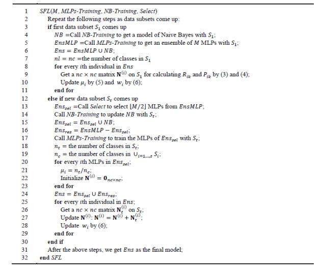
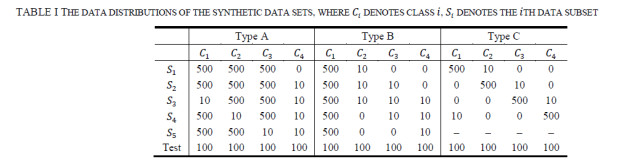
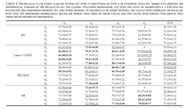
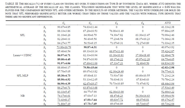
Incremental learning has been investigated by many researchers. However, only few works have considered the situation where class imbalance occurs. In this paper, class imbalanced incremental learning was investigated and an ensemble-based method, named Selective Further Learning (SFL) was proposed. In SFL, a hybrid ensemble of Naive Bayes (NB) and Multilayer Perceptrons (MLPs) were employed. For the ensemble of MLPs, parts of the MLPs were selected to learning from the new data set. Negative Correlation Learning (NCL) with Dynamic Sampling (DyS) for handling class imbalance was used as the basic training method. Besides, as an additive model, Naive Bayes was employed as an individual of the ensemble to learn the data sets incrementally. A group of weights (with the number of the classes as the length) are updated for every individual of the ensemble to indicate the 'confidence' of the individual learning about the classes. The ensemble combines all of the individuals by weighted average according to the weights. Experiments on 3 synthetic data sets and 10 real world data sets showed that SFL was able to handle class imbalance incremental learning and outperform a recently related approach.
Citation: Minlong Lin, Ke Tang. 2017: Selective further learning of hybrid ensemble for class imbalanced increment learning, Big Data and Information Analytics, 2(1): 1-21. doi: 10.3934/bdia.2017005
Incremental learning has been investigated by many researchers. However, only few works have considered the situation where class imbalance occurs. In this paper, class imbalanced incremental learning was investigated and an ensemble-based method, named Selective Further Learning (SFL) was proposed. In SFL, a hybrid ensemble of Naive Bayes (NB) and Multilayer Perceptrons (MLPs) were employed. For the ensemble of MLPs, parts of the MLPs were selected to learning from the new data set. Negative Correlation Learning (NCL) with Dynamic Sampling (DyS) for handling class imbalance was used as the basic training method. Besides, as an additive model, Naive Bayes was employed as an individual of the ensemble to learn the data sets incrementally. A group of weights (with the number of the classes as the length) are updated for every individual of the ensemble to indicate the 'confidence' of the individual learning about the classes. The ensemble combines all of the individuals by weighted average according to the weights. Experiments on 3 synthetic data sets and 10 real world data sets showed that SFL was able to handle class imbalance incremental learning and outperform a recently related approach.

| [1] | A. Asuncion and D. Newman, Uci machine learning repository, 2007. |
| [2] |
Carpenter G. A., Grossberg S., Markuzon N., Reynolds J. H., Rosen D. B. (1992) Fuzzy artmap: A neural network architecture for incremental supervised learning of analog multidimensional maps. IEEE Transactions on Neural Networks 3: 698-713. doi: 10.1109/72.159059

|
| [3] |
G. A. Carpenter, S. Grossberg and J. H. Reynolds,
ARTMAP: Supervised Real-Time Learning and Classification of Nonstationary Data by a Self-Organizing Neural Network Elsevier Science Ltd. , 1991.
10.1109/ICNN.1991.163370 |
| [4] | Chawla N. V., Japkowicz N., Kotcz A. (2004) Editorial: Special issue on learning from imbalanced data sets. Acm Sigkdd Explorations Newsletter 6: 1-6. |
| [5] |
Ditzler G., Muhlbaier M. D., Polikar R. (2010) Incremental learning of new classes in unbalanced datasets: Learn?+?+?.UDNC. International Workshop on Multiple Classifier Systems, Multiple Classifier Systems 33-42. doi: 10.1007/978-3-642-12127-2_4
|
| [6] |
Ditzler G., Polikar R., Chawla N. (2010) An incremental learning algorithm for non-stationary environments and class imbalance. International Conference on Pattern Recognition 2997-3000. doi: 10.1109/ICPR.2010.734
|
| [7] | Freund Y., Schapire R. E. (1999) A short introduction to boosting. Journal of Japanese Society for Artificial Intelligence 14: 771-780. |
| [8] | Fu L., Hsu H.-H., Principe J. C. (1996) Incremental backpropagation learning networks. IEEE Transactions on Neural Networks 7: 757-761. |
| [9] | He H., Garcia E. A. (2009) Learning from imbalanced data. IEEE Transactions on Knowledge and Data Engineering 21: 1263-1284. |
| [10] |
Inoue H., Narihisa H. (2005) Self-organizing neural grove and its applications. IEEE International Joint Conference on Neural Networks 2: 1205-1210. doi: 10.1109/IJCNN.2005.1556025
|
| [11] | N. Japkowicz and S. Stephen, The Class Imbalance Problem: A Systematic Study IOS Press, 2002. |
| [12] |
Kasabov N. (2001) Evolving fuzzy neural networks for supervised/unsupervised online knowledge-based learning. IEEE Transactions on Systems Man & Cybernetics Part B Cybernetics A Publication of the IEEE Systems Man & Cybernetics Society 31: 902-918. doi: 10.1109/3477.969494
|
| [13] | Lin M., Tang K., Yao X. (2013) Dynamic sampling approach to training neural networks for multiclass imbalance classification. IEEE Transactions on Neural Networks and Learning Systems 24: 647-660. |
| [14] | Liu Y., Yao X. (1999) Simultaneous training of negatively correlated neural networks in an ensemble. IEEE Transactions on Systems Man & Cybernetics Part B Cybernetics A Publication of the IEEE Systems Man & Cybernetics Society 29: 716-725. |
| [15] |
Minku F. L., Inoue H., Yao X. (2009) Negative correlation in incremental learning. Natural Computing 8: 289-320. doi: 10.1007/s11047-007-9063-7
|
| [16] |
Muhlbaier M., Topalis A., Polikar R. (2004) Incremental learning from unbalanced data. In
Neural Networks, 2004. Proceedings. 2004 IEEE International Joint Conference on, IEEE 2: 1057-1062. doi: 10.1109/IJCNN.2004.1380080
|
| [17] |
Muhlbaier M., Topalis A., Polikar R. (2004) Learn++.mt: A new approach to incremental learning. Lecture Notes in Computer Science 3077: 52-61. doi: 10.1007/978-3-540-25966-4_5
|
| [18] | M. D. Muhlbaier, A. Topalis and R. Polikar, Learn ++. nc: combining ensemble of classifiers with dynamically weighted consult-and-vote for efficient incremental learning of new classes, IEEE Transactions on Neural Networks 20 (2009), p152. |
| [19] |
Ozawa S., Pang S., Kasabov N. (2008) Incremental learning of chunk data for online pattern classification systems. IEEE Trans Neural Netw 19: 1061-1074. doi: 10.1109/TNN.2007.2000059
|
| [20] |
Polikar R., Byorick J., Krause S., Marino A. (2002) Learn++: A classifier independent incremental learning algorithm for supervised neural networks. International Joint Conference on Neural Networks 1742-1747. doi: 10.1109/IJCNN.2002.1007781
|
| [21] |
Polikar R., Upda L., Upda S. S., Honavar V. (2001) Learn++: an incremental learning algorithm for supervised neural networks. IEEE Transactions on Systems Man & Cybernetics Part C 31: 497-508. doi: 10.1109/5326.983933
|
| [22] |
Salganicoff M. (1997) Tolerating concept and sampling shift in lazy learning using prediction error context switching. Artificial Intelligence Review 11: 133-155. doi: 10.1007/978-94-017-2053-3_5
|
| [23] |
Su M. C., Lee J., Hsieh K. L. (2006) A new artmap-based neural network for incremental learning. Neurocomputing 69: 2284-2300. doi: 10.1016/j.neucom.2005.06.020
|
| [24] |
Sun Y., Kamel M. S., Wang Y. (2006) Boosting for learning multiple classes with imbalanced class distribution. In Data Mining, 2006. ICDM'06. Sixth International Conference on, IEEE 592-602. doi: 10.1109/ICDM.2006.29
|
| [25] |
Tang E. K., Suganthan P. N., Yao X. (2006) An analysis of diversity measures. Machine Learning 65: 247-271. doi: 10.1007/s10994-006-9449-2
|
| [26] |
Tang K., Lin M., Minku F. L., Yao X. (2009) Selective negative correlation learning approach to incremental learning. Neurocomputing 72: 2796-2805. doi: 10.1016/j.neucom.2008.09.022
|
| [27] | Wen W. X., Liu H., Jennings A. (2002) Self-generating neural networks. International Joint Conference on Neural Networks 4: 850-855. |
| [28] |
Widmer G., Kubat M. (1993) Effective learning in dynamic environments by explicit context tracking. In Machine learning: ECML-93, Springer 667: 227-243. doi: 10.1007/3-540-56602-3_139
|
| [29] |
Williamson J. R. (1996) Gaussian artmap: A neural network for fast incremental learning of noisy multidimensional maps. Neural Networks 9: 881-897. doi: 10.1016/0893-6080(95)00115-8
|
Figures(13)

Minlong Lin, Ke Tang. 2017: Selective further learning of hybrid ensemble for class imbalanced increment learning, Big Data and Information Analytics, 2(1): 1-21. doi: 10.3934/bdia.2017005


 DownLoad: