E-commerce user's intention to switch toward drone delivery innovation: The role of environmental concern and customers' attitude

Veronica Veronica; Muhtosim Arief; Asnan Furinto; Lim Sanny; Veronica Veronica; Muhtosim Arief; Asnan Furinto; Lim Sanny

doi:10.3934/environsci.2024042

AIMS Environmental Science

2024, Volume 11, Issue 5: 847-865. doi: 10.3934/environsci.2024042

Previous Article Next Article

Research article

E-commerce user's intention to switch toward drone delivery innovation: The role of environmental concern and customers' attitude

Management Department, BINUS Business School Doctor of Research in Management, Bina Nusantara University, Jakarta, Indonesia 11480

Received: 22 June 2024 Revised: 01 September 2024 Accepted: 25 September 2024 Published: 30 September 2024

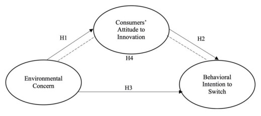
Environmental concern is a determinant in acquiring new green innovation. We aimed to investigate the relationship between environmental concern, consumer attitude, and behavioral intention to switch in the context of drone delivery. The motivation that comes from a green perspective is believed to create a behavior that is also keen on innovative green products. One of the examples is the implementation of drones in delivering parcels, which is believed to cut the carbon footprint. Our purpose was to analyze the direct impact of environmental concern on consumers' behavioral intentions regarding e-commerce drone delivery. Additionally, we aimed to examine the mediating role of consumers' attitudes toward innovation in the relationship between environmental concern and behavioral intention. We sought to provide insights into how environmental awareness and the adoption of innovative delivery technologies like drones can influence consumer behavior, contributing to more sustainable and eco-friendly e-commerce practices. Structured questionnaires were provided to e-commerce users, reliability and validity tests were confirmed, and structural equation modeling (SEM) was used to analyze the relationships among variables. The results of the SEM analysis proved that environmental concern and consumer attitudes have a positive impact on behavioral intention. Customer attitude mediates the relationship between environmental concern and behavioral intention. This research provides a deeper understanding of how environmental concerns influence consumer behavior towards drone delivery innovation within the e-commerce sector. The implications integrate environmental concerns with consumer behavior and innovation adoption, providing a comprehensive view that goes beyond traditional marketing and consumer research.
- Drones delivery,
- environmental concern,
- attitude,
- consumer innovativeness,
- innovation
Citation: Veronica Veronica, Muhtosim Arief, Asnan Furinto, Lim Sanny. E-commerce user's intention to switch toward drone delivery innovation: The role of environmental concern and customers' attitude[J]. AIMS Environmental Science, 2024, 11(5): 847-865. doi: 10.3934/environsci.2024042

Related Papers:

Abstract

Environmental concern is a determinant in acquiring new green innovation. We aimed to investigate the relationship between environmental concern, consumer attitude, and behavioral intention to switch in the context of drone delivery. The motivation that comes from a green perspective is believed to create a behavior that is also keen on innovative green products. One of the examples is the implementation of drones in delivering parcels, which is believed to cut the carbon footprint. Our purpose was to analyze the direct impact of environmental concern on consumers' behavioral intentions regarding e-commerce drone delivery. Additionally, we aimed to examine the mediating role of consumers' attitudes toward innovation in the relationship between environmental concern and behavioral intention. We sought to provide insights into how environmental awareness and the adoption of innovative delivery technologies like drones can influence consumer behavior, contributing to more sustainable and eco-friendly e-commerce practices. Structured questionnaires were provided to e-commerce users, reliability and validity tests were confirmed, and structural equation modeling (SEM) was used to analyze the relationships among variables. The results of the SEM analysis proved that environmental concern and consumer attitudes have a positive impact on behavioral intention. Customer attitude mediates the relationship between environmental concern and behavioral intention. This research provides a deeper understanding of how environmental concerns influence consumer behavior towards drone delivery innovation within the e-commerce sector. The implications integrate environmental concerns with consumer behavior and innovation adoption, providing a comprehensive view that goes beyond traditional marketing and consumer research.

References

[1]	Statista (2023) E-commerce in Indonesia-statistics & Facts. Available from: https://www.statista.com/topics/5742/e-commerce-in-indonesia/#topicOverview.
[2]	AJ Marketing (2023) Indonesia ecommerce market: Data, trends, top stories. Available from: https://www.indonesia-investments.com/business/business-columns/indonesia-ecommerce-market-data-trends-top-stories/item9630.
[3]	Allen J, Piecyk M, Piotrowska M, et al. (2018) Understanding the impact of e-commerce on last-mile light goods vehicle activity in urban areas: The case of London. Transport Res D Tr E 61: 325–338. https://doi.org/10.1016/j.trd.2017.07.020 doi: 10.1016/j.trd.2017.07.020
[4]	Mangiaracina R, Perego A, Seghezzi A, et al. (2019) Innovative solutions to increase last-mile delivery efficiency in B2C e-commerce: A literature review. Int J Phys Distr Log 49: 901–920. https://doi.org/10.1108/IJPDLM-02-2019-0048 doi: 10.1108/IJPDLM-02-2019-0048
[5]	Anvari R (2023) Green, closed loop, and reverse supply chain: A literature review. J Bus Manag 1: 33–57. https://doi.org/10.47747/jbm.v1i1.956 doi: 10.47747/jbm.v1i1.956
[6]	Chen C, Pan S (2016) Using the crowd of taxis to last mile delivery in E-commerce: A methodological research. Serv Orientat Holonic Multi-Ag Manufact 61–70. https://doi.org/10.1007/978-3-319-30337-6_6 doi: 10.1007/978-3-319-30337-6_6
[7]	Anvari R, Askari KOA (2024) Evaluating the efficiency of resource and energy consumption of farmland systems. SSRN Electron J. https://dx.doi.org/10.2139/ssrn.4761505 doi: 10.2139/ssrn.4761505
[8]	Lavanya R (2016) The 2015 Paris agreement: Interplay between hard, soft and non-obligations. J Environ law 28: 337–358. https://www.jstor.org/stable/26168923
[9]	Rogelj J, Elzen MD, Hö hne N, et al. (2016) Paris Agreement climate proposals need a boost to keep warming well below 2 ℃. Nature 534: 631–639. https://doi.org/10.1038/nature18307 doi: 10.1038/nature18307
[10]	Maitreyee D, Rangarajan K (2020) Impact of policy initiatives and collaborative synergy on sustainability and business growth of Indian SMEs. Indian Growth Dev Rev 13: 607–627. https://doi.org/10.1108/IGDR-09-2019-0095 doi: 10.1108/IGDR-09-2019-0095
[11]	Muangmee C, Pikiewicz ZD, Meekaewkunchorn N, et al. (2021) Green entrepreneurial orientation and green innovation in small and medium-sized enterprises (Smes). Soc Sci 10: 2021. https://doi.org/10.3390/socsci10040136 doi: 10.3390/socsci10040136
[12]	Raj A, Sah B (2019) Analyzing critical success factors for implementation of drones in the logistics sector using grey-DEMATEL based approach. Comput Ind Eng 138: 106118. https://doi.org/10.1016/j.cie.2019.106118 doi: 10.1016/j.cie.2019.106118
[13]	Kellermann R, Biehle T, Fischer L (2020) Drones for parcel and passenger transportation: A literature review. Transp Res Interdisc 4: 100088. https://doi.org/10.1016/j.trip.2019.100088 doi: 10.1016/j.trip.2019.100088
[14]	Cam LNT (2023) A rising trend in eco-friendly products: A health-conscious approach to green buying. Heliyon 9: e19845. https://doi.org/10.1016/j.heliyon.2023.e19845 doi: 10.1016/j.heliyon.2023.e19845
[15]	Mahesh S, Ramadurai G, Nagendra SMS (2019) Real-world emissions of gaseous pollutants from motorcycles on Indian urban arterials. Transport Res D Tr E 76: 72–84. https://doi.org/10.1016/j.trd.2019.09.010 doi: 10.1016/j.trd.2019.09.010
[16]	Mathew AO, Jha AN, Lingappa AK, et al. (2021) Attitude towards drone food delivery services—role of innovativeness, perceived risk, and green image. J Open Innov Technol Mark Complex 7: 144. https://doi.org/10.3390/joitmc7020144 doi: 10.3390/joitmc7020144
[17]	Dileep MR, Navaneeth AV, Ullagaddi S, et al. (2020) A study and analysis on various types of agricultural drones and its applications, in 2020 Fifth International Conference on Research in Computational Intelligence and Communication Networks, 181–185. https://doi.org/10.1109/ICRCICN50933.2020.9296195
[18]	Puri V, Nayyar A, Raja L (2017) Agriculture drones: A modern breakthrough in precision agriculture. J Stat Manag Syst 20: 507–518. https://doi.org/10.1080/09720510.2017.1395171 doi: 10.1080/09720510.2017.1395171
[19]	Nwaogu JM, Yang Y, Chan AP, et al. (2023) Application of drones in the architecture, engineering, and construction (AEC) industry. Automat Constr 150. https://doi.org/10.1016/j.autcon.2023.104827 doi: 10.1016/j.autcon.2023.104827
[20]	Goodchild A, Toy J (2018) Delivery by drone: An evaluation of unmanned aerial vehicle technology in reducing CO₂ emissions in the delivery service industry. Transport Res D Tr E 61: 58–67. https://doi.org/10.1016/j.trd.2017.02.017 doi: 10.1016/j.trd.2017.02.017
[21]	Clutch (2020) Drone delivery: Benefits and challenges. Available from: https://clutch.co/logistics/resources/drone-delivery-statistics-benefits-challenges.
[22]	Hwang J, Choe JY (2019) Exploring perceived risk in building successful drone food delivery services. Int J Contemp Hosp M 31: 3249–3269. https://doi.org/10.1108/IJCHM-07-2018-0558 doi: 10.1108/IJCHM-07-2018-0558
[23]	Yoo W, Yu E, Jung J (2018) Drone delivery: Factors affecting the public's attitude and intention to adopt. Telemat Inform 35: 1687–1700. https://doi.org/10.1016/j.tele.2018.04.014 doi: 10.1016/j.tele.2018.04.014
[24]	Hu ZH, Huang YL, Li YN, et al. (2024) Drone-based instant delivery hub-and-spoke network optimization. Drones 8. https://doi.org/10.3390/drones8060247 doi: 10.3390/drones8060247
[25]	Chiang WC, Li Y, Shang J, et al. (2019) Impact of drone delivery on sustainability and cost: Realizing the UAV potential through vehicle routing optimization. Appl Energy 242: 1164–1175. https://doi.org/10.1016/j.apenergy.2019.03.117 doi: 10.1016/j.apenergy.2019.03.117
[26]	Adnan N, Nordin SM, Rahman I, et al. (2017) A new era of sustainable transport: An experimental examination on forecasting adoption behavior of EVs among Malaysian consumer. Transport Res A-Pol 103: 279–295. https://doi.org/10.1016/j.tra.2017.06.010 doi: 10.1016/j.tra.2017.06.010
[27]	Baeshen Y, Soomro YA, Bhutto MY (2021) Determinants of green innovation to achieve sustainable business performance: Evidence from SMEs. Front Psychol 12: 767968. https://doi.org/10.3389/fpsyg.2021.767968 doi: 10.3389/fpsyg.2021.767968
[28]	Rodrigues TA, Patrikar J, Oliveira NL, et al. (2022) Drone flight data reveal energy and greenhouse gas emissions savings for very small package delivery. Patterns 3: 100569. https://doi.org/10.1016/j.patter.2022.100569 doi: 10.1016/j.patter.2022.100569
[29]	Balderjahn I (1988) Personality variables and environmental attitudes as predictors of ecologically responsible consumption patterns. J Bus Res 17: 51–56. https://doi.org/10.1016/0148-2963(88)90022-7 doi: 10.1016/0148-2963(88)90022-7
[30]	Crosby LA, Taylor JR (1982) Consumer satisfaction with Michigan's container deposit law: An ecological perspective. J Mark 46: 47–60. https://doi.org/10.2307/1251159 doi: 10.2307/1251159
[31]	Thieme J, Royne MB, Jha S, et al. (2015) Factors affecting the relationship between environmental concern and behaviors. Mark Intell Plan 33: 675–690. https://doi.org/10.1108/MIP-08-2014-0149 doi: 10.1108/MIP-08-2014-0149
[32]	Ozaki R, Sevastyanova K (2011) Going hybrid: An analysis of consumer purchase motivations. Energy Policy 39: 2217–2227. https://doi.org/10.1016/j.enpol.2010.04.024 doi: 10.1016/j.enpol.2010.04.024
[33]	Teoh CW, Gaur SS (2019) Environmental concern: An issue for poor or rich. Manag Environ Qual 30: 227–242. https://doi.org/10.1108/MEQ-02-2018-0046 doi: 10.1108/MEQ-02-2018-0046
[34]	Bamberg S (2003) How does environmental concern influence specific environmentally related behaviors? A new answer to an old question. J Environ Psychol 23: 21–32. https://doi.org/10.1016/S0272-4944(02)00078-6 doi: 10.1016/S0272-4944(02)00078-6
[35]	Stafford MR, Stafford TF, Collier JE (2006) The dimensionality of environmental concern: Validation of component measures. Interdiscip Environ Rev 8: 43–61. https://doi.org/10.1504/IER.2006.053946 doi: 10.1504/IER.2006.053946
[36]	Ajzen I (1991) The theory of planned behavior. Organ Behav Hum Dec 50: 179–211. https://doi.org/10.1016/0749-5978(91)90020-T doi: 10.1016/0749-5978(91)90020-T
[37]	Schiffman LG, Kanuk LL (2004) Consumer behavior, 8th International Edition, Prentice Hall.
[38]	Kotler P, (2009) Marketing management, Jakarta: Erlangga.
[39]	Hawkins DI, Mothersbaugh DL (2013) Consumer behavior: Building marketing strategy, New York: McGraw-Hill Irwin.
[40]	Crosby LA, Gill JD, Taylor JR (1981) Consumer voter behavior in the passage of the Michigan container law. J Mark 45: 19–32. https://doi.org/10.1177/002224298104500203 doi: 10.1177/002224298104500203
[41]	Bettencourt LA, Hughner RS, Kuntze RJ, et al. (1999) Lifestyle of the tight and frugal: Theory and measurement. J Consum Res 26: 85–99. https://doi.org/10.1086/209552 doi: 10.1086/209552
[42]	Schiffman LG, Wisenblit J (2015) Consumer behavior, England: Pearson Education Limited, 2015.
[43]	Agarwal J, Malhotra NK (2005) An integrated model of attitude and affect: Theoretical foundation and an empirical investigation. J Bus Res 58: 483–493. https://doi.org/10.1016/S0148-2963(03)00138-3 doi: 10.1016/S0148-2963(03)00138-3
[44]	Reaños MAT, Meier D, Curtis J, et al. (2023) The role of energy, financial attitudes and environmental concerns on perceived retrofitting benefits and barriers: Evidence from Irish home owners. Energy Buildings 297: 113448. https://doi.org/10.1016/j.enbuild.2023.113448 doi: 10.1016/j.enbuild.2023.113448
[45]	De Groot J, Steg L (2007) General beliefs and the theory of planned behavior: The role of environmental concerns in the TPB. J Appl Soc Psychol 37: 1817–1836. https://doi.org/10.1111/j.1559-1816.2007.00239.x doi: 10.1111/j.1559-1816.2007.00239.x
[46]	Lau JL, Hashim AH (2020) Mediation analysis of the relationship between environmental concern and intention to adopt green concepts. Smart Sustain Built 9: 539–556. https://doi.org/10.1108/SASBE-09-2018-0046 doi: 10.1108/SASBE-09-2018-0046
[47]	Li D, Zhao L, Ma S, et al. (2019) What influences an individual's pro-environmental behavior? A literature review. Resour Conserv Recy 146: 28–34. https://doi.org/10.1016/j.resconrec.2019.03.024 doi: 10.1016/j.resconrec.2019.03.024
[48]	Jaiswal D, Kaushal V, Kant R, et al. (2021) Consumer adoption intention for electric vehicles: Insights and evidence from Indian sustainable transportation. Technol Forecast Soc 173: 121089. https://doi.org/10.1016/j.techfore.2021.121089 doi: 10.1016/j.techfore.2021.121089
[49]	Yue B, Sheng G, She S, et al. (2020) Impact of consumer environmental responsibility on green consumption behavior in China: The role of environmental concern and price sensitivity. Sustainability 12. https://doi.org/10.3390/su12052074 doi: 10.3390/su12052074
[50]	SIRCLO (2021) Navigating Indonesia's e-commerce: Omnichannel as the future of retail. Available from: https://www.sirclo.com/research-reports/navigating-indonesia-s-e-commerce-omnichannel-as-the-future-of-retail.
[51]	Sekaran U, Bougie R (2016) Research methods for business: A skill-building approach, 7 Eds., Chichester, West Sussex, United Kingdom: John Wiley & Sons.
[52]	Bentler PM, Chou CP (1987) Practical issues in structural modeling. Sociol Method Res 16: 78–117. https://doi.org/10.1177/0049124187016001004 doi: 10.1177/0049124187016001004
[53]	Nunnally JC, Bernstein IH (1967) Psychometric theory, New York: McGraw-Hill.

Reader Comments

Your name:*

Email:*
© 2024 the Author(s), licensee AIMS Press. This is an open access article distributed under the terms of the Creative Commons Attribution License (http://creativecommons.org/licenses/by/4.0)