Analysis of Data Splitting on Streamflow Prediction using Random Forest

Diksha Puri; Parveen Sihag; Mohindra Singh Thakur; Mohammed Jameel; Aaron Anil Chadee; Mohammad Azamathulla Hazi; Diksha Puri; Parveen Sihag; Mohindra Singh Thakur; Mohammed Jameel; Aaron Anil Chadee; Mohammad Azamathulla Hazi

doi:10.3934/environsci.2024029

AIMS Environmental Science

2024, Volume 11, Issue 4: 593-609. doi: 10.3934/environsci.2024029

Previous Article Next Article

Research Article Special Issues

Analysis of Data Splitting on Streamflow Prediction using Random Forest

1.
School of Environmental Science, Shoolini University, Solan, Himachal Pradesh, 173229, India (dikshapuri10@gmail.com)
2.
Department of Civil Engineering, Chandigarh University, Punjab 140301, India (parveen12sihag@gmail.com)
3.
Department of Civil Engineering, Shoolini University, Solan, Himachal Pradesh, 173229, India (mohindrasinghthakur@shooliniuniversity.com)
4.
Department of Civil Engineering, King Khalid University, Abha, Saudi Arabia (jamoali@kku.edu.sa)
5.
Department of Civil and Environmental Engineering, University of the West Indies, Trinidad

Received: 07 June 2024 Revised: 13 July 2024 Accepted: 17 July 2024 Published: 26 July 2024

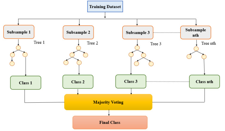
This study is focused on the use of random forest (RF) to forecast the streamflow in the Kesinga River basin. A total of 169 data points were gathered monthly for the years 1991–2004 to create a model for streamflow prediction. The dataset was allotted into training and testing stages using various ratios, such as 50/50, 60/40, 70/30, and 80/20. The produced models were evaluated using three statistical indices: the root mean square error (RMSE), the mean absolute error (MAE), and the correlation coefficient (CC). The analysis of the models' performances revealed that the training and testing ratios had a substantial impact on the RF model's predictive abilities; models performed best when the ratio was 60/40. The findings demonstrated the right dataset ratios for precise streamflow prediction, which will be beneficial for hydraulic engineers during the water-related design and engineering stages of water projects.
- streamflow prediction,
- Kesinga basin,
- data separation ratios,
- random forest,
- 60/40
Citation: Diksha Puri, Parveen Sihag, Mohindra Singh Thakur, Mohammed Jameel, Aaron Anil Chadee, Mohammad Azamathulla Hazi. Analysis of Data Splitting on Streamflow Prediction using Random Forest[J]. AIMS Environmental Science, 2024, 11(4): 593-609. doi: 10.3934/environsci.2024029

Related Papers:

Abstract

This study is focused on the use of random forest (RF) to forecast the streamflow in the Kesinga River basin. A total of 169 data points were gathered monthly for the years 1991–2004 to create a model for streamflow prediction. The dataset was allotted into training and testing stages using various ratios, such as 50/50, 60/40, 70/30, and 80/20. The produced models were evaluated using three statistical indices: the root mean square error (RMSE), the mean absolute error (MAE), and the correlation coefficient (CC). The analysis of the models' performances revealed that the training and testing ratios had a substantial impact on the RF model's predictive abilities; models performed best when the ratio was 60/40. The findings demonstrated the right dataset ratios for precise streamflow prediction, which will be beneficial for hydraulic engineers during the water-related design and engineering stages of water projects.

References

[1]	Yang D, Yang Y, Xia, J (2021) Hydrological cycle and water resources in a changing world: A review. Geogr Sustain 2: 115–122. https://doi.org/10.1016/j.geosus.2021.05.003 doi: 10.1016/j.geosus.2021.05.003
[2]	Liang, S, Ge, S, Wan, L., & Zhang, J. (2010). Can climate change cause the Yellow River to dry up? Water Resour Res 46 https://doi.org/10.1029/2009WR007971 doi: 10.1029/2009WR007971
[3]	L Mampitiya, N Rathnayake, Y Hoshino et al. (2024). Forecasting PM10 Levels in Sri Lanka: A Comparative Analysis of Machine Learning Models. J Hazard Mater Adv 13: 1–10
[4]	HI Tillekaratne, IMSP Jayawardena, V Basnayaka, et al. (2023) Hydro-meteorological disaster incidents and associated weather systems in Sri Lanka. J Environ Informatics Lett 10: 89–103.
[5]	M Fuladipanah, A Shahhosseini, N Rathnayake, et al. (2024) In-depth simulation of rainfall-runoff relationships using machine learning methods. Water Pract Technol (In-Press).
[6]	Palmer M, Ruhi A (2019) Linkages between flow regime, biota, and ecosystem processes: Implications for river restoration. Science 365: eaaw2087.
[7]	Bierkens, MF, Wada, Y (2019) Non-renewable groundwater use and groundwater depletion: a review. Environ Res Lett 14: 063002. https://doi.org/10.1088/1748-9326/ab1a5f doi: 10.1088/1748-9326/ab1a5f
[8]	Zhou Y, Ma J, Zhang Y, et al. (2019) Influence of the three Gorges Reservoir on the shrinkage of China's two largest freshwater lakes. Global Planet Change 177: 45–55. https://doi.org/10.1016/j.gloplacha.2019.03.014 doi: 10.1016/j.gloplacha.2019.03.014
[9]	Adamowski J. F (2008) Development of a short-term river flood forecasting method for snowmelt driven floods based on wavelet and cross-wavelet analysis. J Hydrol 353: 247–266.
[10]	Vorosmarty CJ, Green P, Salisbury J, et al. (2000) Global water resources: vulnerability from climate change and population growth. Science 289: 284–288. https://doi.org/10.1126/science.289.5477.284 doi: 10.1126/science.289.5477.284
[11]	Hanson RT, Newhouse MW, Dettinger, MD (2004) A methodology to asess relations between climatic variability and variations in hydrologic time series in the southwestern United States. J Hydrol 287: 252–269. https://doi.org/10.1016/j.jhydrol.2003.10.006 doi: 10.1016/j.jhydrol.2003.10.006
[12]	Yang C, Lin Z, Yu Z, et al. (2010) Analysis and simulation of human activity impact on streamflow in the Huaihe River basin with a large-scale hydrologic model. J Hydrometeorol 11: 810–821. https://doi.org/10.1175/2009JHM1145.1 doi: 10.1175/2009JHM1145.1
[13]	Makumbura RK, Rathnayake U (2022) Variation of Leaf Area Index (LAI) under changing climate: Kadolkele mangrove forest, Sri Lanka, Advances in Meteorology.
[14]	Labat D, Ababou R, Mangin A (2000) Rainfall–runoff relations for karstic springs. Part Ⅱ: continuous wavelet and discrete orthogonal multiresolution analyses. J Hydrol 238: 149–178.
[15]	Coulibaly P, Burn DH (2004) Wavelet analysis of variability in annual Canadian streamflows. Water Resour Res 40. https://doi.org/10.1029/2003WR002667 doi: 10.1029/2003WR002667
[16]	Guven A (2009) Linear genetic programming for time-series modelling of daily flow rate. J Earth Syst Sci 118: 137–146. https://doi.org/10.1007/s12040-009-0022-9 doi: 10.1007/s12040-009-0022-9
[17]	Yaseen ZM, El-Shafie A, Jaafar O, et al. (2015) Artificial intelligence-based models for stream-flow forecasting: 2000–2015. J Hydrol 530: 829–844. https://doi.org/10.1016/j.jhydrol.2015.10.038 doi: 10.1016/j.jhydrol.2015.10.038
[18]	SP Hemakumara, MB Gunathilake, U Rathnayake (2023) Flow alterations due a constructed reservoir in the Menik Ganga basin, Sri Lanka. Discover Water 3: 1–15.
[19]	Ghimire S, Yaseen ZM, Farooque AA, et al. (2021). Streamflow prediction using an integrated methodology based on convolutional neural network and long short-term memory networks. Sci Rep 11: 17497.
[20]	Liu D, Jiang W, Mu L, et al. (2020) Streamflow prediction using deep learning neural network: case study of Yangtze River. IEEE access 8: 90069–90086.
[21]	Arsenault R, Martel JL, Brunet F, et al. (2023) Continuous streamflow prediction in ungauged basins: long short-term memory neural networks clearly outperform traditional hydrological models. Hydrol Earth Syst Sci 27: 139–157.
[22]	Tabbussum R, Dar AQ (2021) Comparison of fuzzy inference algorithms for stream flow prediction. Neural Comput Appl 33: 1643–1653.
[23]	Üneş F, Demirci M, Zelenakova M, et al. (2020) River flow estimation using artificial intelligence and fuzzy techniques. Water 12: 2427. https://doi.org/10.3390/w12092427 doi: 10.3390/w12092427
[24]	Mohammadi B, Linh NTT, Pham QB, et al. (2020) Adaptive neuro-fuzzy inference system coupled with shuffled frog leaping algorithm for predicting river streamflow time series. Hydrol Sci J 65: 1738–1751. https://doi.org/10.1080/02626667.2020.1758703 doi: 10.1080/02626667.2020.1758703
[25]	Di Nunno F, de Marinis G, Granata, F. (2023) Short-term forecasts of streamflow in the UK based on a novel hybrid artificial intelligence algorithm. Sci Rep 13: 7036.
[26]	Tikhamarine Y, Souag-Gamane D, Ahmed AN, et al. (2020) Improving artificial intelligence models accuracy for monthly streamflow forecasting using grey Wolf optimization (GWO) algorithm. J Hydrol 582: 124435. https://doi.org/10.1016/j.jhydrol.2019.124435 doi: 10.1016/j.jhydrol.2019.124435
[27]	Seidu J, Ewusi A, Kuma JSY, et al. (2023) Impact of data partitioning in groundwater level prediction using artificial neural network for multiple wells. Int J River Basin Ma 21: 639–650. https://doi.org/10.1080/15715124.2022.2079653 doi: 10.1080/15715124.2022.2079653
[28]	Jahanpanah E, Khosravinia P, Sanikhani H, et al. (2019) Estimation of discharge with free overfall in rectangular channel using artificial intelligence models. Flow Meas Instrum 67: 118–130. https://doi.org/10.1016/j.flowmeasinst.2019.04.005 doi: 10.1016/j.flowmeasinst.2019.04.005
[29]	Demir S, Sahin EK (2022) Comparison of tree-based machine learning algorithms for predicting liquefaction potential using canonical correlation forest, rotation forest, and random forest based on CPT data. Soil Dyn Earthq Eng 154: 107130. https://doi.org/10.1016/j.soildyn.2021.107130 doi: 10.1016/j.soildyn.2021.107130
[30]	Ebtehaj I, Bonakdari H, Safari MJS, et al. (2020) Combination of sensitivity and uncertainty analyses for sediment transport modeling in sewer pipes. Int J Sediment Res 35: 157–170. https://doi.org/10.1016/j.ijsrc.2019.08.005 doi: 10.1016/j.ijsrc.2019.08.005
[31]	Zhang W, Zhang R, Wu C, et al. (2020) State-of-the-art review of soft computing applications in underground excavations. Geosci Front 11: 1095–1106. https://doi.org/10.1016/j.gsf.2019.12.003 doi: 10.1016/j.gsf.2019.12.003
[32]	Xu Z, Sheykhahmad FR, Ghadimi N, et al. (2020) Computer-aided diagnosis of skin cancer based on soft computing techniques. Open Med 15: 860–871. https://doi.org/10.1515/med-2020-0131 doi: 10.1515/med-2020-0131
[33]	Al-Janabi S, Mohammad M, Al-Sultan A (2020) A new method for prediction of air pollution based on intelligent computation. Soft Comput 24: 661–680.
[34]	Wang F, Chun W, Cui, Y (2022) Urban water resources allocation and low-carbon economic development based on soft computing. Environ Technol Inno 28: 102292. https://doi.org/10.1016/j.eti.2022.102292 doi: 10.1016/j.eti.2022.102292
[35]	Luan C, Liu R, Peng S (2021) Land-use suitability assessment for urban development using a GIS-based soft computing approach: A case study of Ili Valley, China. Ecol Indic 123: 107333. https://doi.org/10.1016/j.ecolind.2020.107333 doi: 10.1016/j.ecolind.2020.107333
[36]	Asteris PG, Apostolopoulou M, Armaghani DJ, et al. (2020). On the metaheuristic models for the prediction of cement-metakaolin mortars compressive strength. 1: 063
[37]	Breiman L (2001) Random forests. Mach Learn 45: 5–32.
[38]	Liaw A, Wiener M (2002) Classification and regression by randomForest. R News 2: 18–22.
[39]	Scornet E, Biau G, Vert JP (2015). Consistency of random forests.
[40]	Mohanty S, Roy N, Singh SP, et al. (2019). Estimating the strength of stabilized dispersive soil with cement clinker and fly ash. Geotech Geol Eng 37: 2915–2926.
[41]	Breiman L (1996) Bagging predictors. Mach Learn 24: 123–140.
[42]	Egawa, T, Suzuki K, Ichikawa Y, et al. (2011, July) A water flow forecasting for dam using neural networks and regression models. In 2011 IEEE Power and Energy Society General Meeting (1–6). IEEE. https://doi.org/10.1109/PES.2011.6038925
[43]	AlOmar M. K, Khaleel F, AlSaadi A. A, et al. (2022) The influence of data length on the performance of artificial intelligence models in predicting air pollution. Adv Meteorol 2022. https://doi.org/10.1155/2022/5346647
[44]	Polat K, Akdemir B, Güneş S (2008) Computer aided diagnosis of ECG data on the least square support vector machine. Digit Signal Process 18: 25–32.
[45]	Bui D. T, Pradhan B, Lofman O, et al. (2012) Landslide susceptibility mapping at Hoa Binh province (Vietnam) using an adaptive neuro-fuzzy inference system and GIS. Comput Geosci 45: 199–211. https://doi.org/10.1016/j.cageo.2011.10.031 doi: 10.1016/j.cageo.2011.10.031
[46]	Huang F, Yin K, Huang J, et al. (2017) Landslide susceptibility mapping based on self-organizing-map network and extreme learning machine. Engineering Geology 223: 11–22. https://doi.org/10.1016/j.enggeo.2017.04.013 doi: 10.1016/j.enggeo.2017.04.013
[47]	Pham B. T, Tien Bui D, Pourghasemi H. R, et al. (2017) Landslide susceptibility assesssment in the Uttarakhand area (India) using GIS: a comparison study of prediction capability of naï ve bayes, multilayer perceptron neural networks, and functional trees methods. Theor Appl Climatol 128: 255–273.
[48]	Khasawneh N, Fraiwan M, Fraiwan L. (2023) Detection of K-complexes in EEG signals using deep transfer learning and YOLOv3. Cluster Comput 26: 3985–3995.
[49]	Kaur R, Kumar R, Gupta, M (2022) Predicting risk of obesity and meal planning to reduce the obesity in adulthood using artificial intelligence. Endocrine 78: 458–469.
[50]	Ikram R. M. A, Dai H. L, Ewees A. A, et al. (2022) Application of improved version of multi verse optimizer algorithm for modeling solar radiation. Energy Rep 8: 12063–12080. https://doi.org/10.1016/j.egyr.2022.09.015 doi: 10.1016/j.egyr.2022.09.015
[51]	Shirzadi A, Solaimani K, Roshan M. H, et al. (2019) Uncertainties of prediction accuracy in shallow landslide modeling: Sample size and raster resolution. Catena 178: 172–188.
[52]	Kulkarni S (2023, November) Impact of Various Data Splitting Ratios on the Performance of Machine Learning Models in the Classification of Lung Cancer. In Proceedings of the Second International Conference on Emerging Trends in Engineering (ICETE 2023) (223: 96). Springer Nature.
[53]	Kisi O, Mirboluki A, Naganna S. R, et al. (2022) Comparative evaluation of deep learning and machine learning in modelling pan evaporation using limited inputs. Hydrol Sci J 67: 1309–1327.

Reader Comments

Your name:*

Email:*
© 2024 the Author(s), licensee AIMS Press. This is an open access article distributed under the terms of the Creative Commons Attribution License (http://creativecommons.org/licenses/by/4.0)