An exact solution of heat and mass transfer analysis on hydrodynamic magneto nanofluid over an infinite inclined plate using Caputo fractional derivative model

J. Kayalvizhi; A. G. Vijaya Kumar; Ndolane Sene; Ali Akgül; Mustafa Inc; Hanaa Abu-Zinadah; S. Abdel-Khalek; J. Kayalvizhi; A. G. Vijaya Kumar; Ndolane Sene; Ali Akgül; Mustafa Inc; Hanaa Abu-Zinadah; S. Abdel-Khalek

doi:10.3934/math.2023180

AIMS Mathematics

2023, Volume 8, Issue 2: 3542-3560. doi: 10.3934/math.2023180

Previous Article Next Article

Research article Special Issues

An exact solution of heat and mass transfer analysis on hydrodynamic magneto nanofluid over an infinite inclined plate using Caputo fractional derivative model

1.
Department of Mathematics, School of Advanced Sciences Vellore Institute of Technology, Vellore-632014, India
2.
Department of Mathematics, Institut des Politiques Publiques, Cheikh Anta Diop University, Dakar Fann, Senegal
3.
Siirt University, Art and Science Faculty, Department of Mathematics, 56100 Siirt, Turkey
4.
Near East University, Mathematics Research Center, Department of Mathematics, Near East Boulevard, PC: 99138, Nicosia/Mersin 10-Turkey
5.
Department of Mathematics, Science Faculty, Firat University, 23119 Elazig, Turkey
6.
Department of Medical Research, China Medical University, 40402 Taichung, Taiwan
7.
University of Jeddah, College of Science, Department of Statistics, Jeddah, Saudi Arabia
8.
Department of Mathematics, College of Science, Taif University, P.O. Box 11099, Taif 21944, Saudi Arabia

Received: 26 June 2022 Revised: 12 October 2022 Accepted: 12 October 2022 Published: 22 November 2022
MSC : 35Q30, 26A33

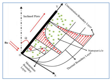
This paper presents the problem modeled using Caputo fractional derivatives with an accurate study of the MHD unsteady flow of Nanofluid through an inclined plate with the mass diffusion effect in association with the energy equation. H₂O is thought to be a base liquid with clay nanoparticles floating in it in a uniform way. Bousinessq's approach is used in the momentum equation for pressure gradient. The nondimensional fluid temperature, species concentration, and fluid transport are derived together with Jacob Fourier sine and Laplace transforms Techniques in terms of exponential decay function, whose inverse is computed further in terms of Mittag-Leffler function. The impact of various physical quantities interpreted with fractional order of the Caputo derivatives. The obtained temperature, transport, and species concentration profiles show behaviours for $0 < \mathtt{α} < 1$ where $\mathtt{α} $ is the fractional parameter. Numerical calculations have been carried out for the rate of heat transmission and the Sherwood number is swotted to be put in the form of tables. The parameters for the magnetic field and the angle of inclination slow down the boundary layer of momentum. The distributions of velocity, temperature, and concentration expand more rapidly for higher values of the fractional parameter. Additionally, it is revealed that for the volume fraction of nanofluids, the concentration profiles behave in the opposite manner. The limiting case solutions also presented on flow field of governing model.
- nanofluid,
- heat and mass transfer,
- magnetic field,
- Caputo fractional derivative,
- Fourier and integral transforms
Citation: J. Kayalvizhi, A. G. Vijaya Kumar, Ndolane Sene, Ali Akgül, Mustafa Inc, Hanaa Abu-Zinadah, S. Abdel-Khalek. An exact solution of heat and mass transfer analysis on hydrodynamic magneto nanofluid over an infinite inclined plate using Caputo fractional derivative model[J]. AIMS Mathematics, 2023, 8(2): 3542-3560. doi: 10.3934/math.2023180

Related Papers:

Abstract

This paper presents the problem modeled using Caputo fractional derivatives with an accurate study of the MHD unsteady flow of Nanofluid through an inclined plate with the mass diffusion effect in association with the energy equation. H₂O is thought to be a base liquid with clay nanoparticles floating in it in a uniform way. Bousinessq's approach is used in the momentum equation for pressure gradient. The nondimensional fluid temperature, species concentration, and fluid transport are derived together with Jacob Fourier sine and Laplace transforms Techniques in terms of exponential decay function, whose inverse is computed further in terms of Mittag-Leffler function. The impact of various physical quantities interpreted with fractional order of the Caputo derivatives. The obtained temperature, transport, and species concentration profiles show behaviours for $0 < \mathtt{α} < 1$ where $\mathtt{α} $ is the fractional parameter. Numerical calculations have been carried out for the rate of heat transmission and the Sherwood number is swotted to be put in the form of tables. The parameters for the magnetic field and the angle of inclination slow down the boundary layer of momentum. The distributions of velocity, temperature, and concentration expand more rapidly for higher values of the fractional parameter. Additionally, it is revealed that for the volume fraction of nanofluids, the concentration profiles behave in the opposite manner. The limiting case solutions also presented on flow field of governing model.

References

[1]	S. U. S. Choi, J. A. Eastman, Enhancing thermal conductivity of fluids with nanoparticles, Conference: International mechanical engineering congress and exhibition, San Francisco, CA, 1995, 12–17.
[2]	V. W. Kaufui, D. L. Omar, Applications of nanofluids: Current and future, Adv. Mech. Eng., 11 (2010), 105–132.
[3]	O. Mahian, L. Kolsi, M. Amani, P. Estellé, G. Ahmadi, C. Kleinstreuer, et al., Recent advances in modeling and simulation of nanofluid flows-Part I: Fundamentals and theory, Phys. Rep., 790 (2019), 1–48. https://doi.org/10.1016/j.physrep.2018.11.004
[4]	J. A. Eastman, U. S. Choi, S. P. Li, L. J. Thompson, S. Lee, Enhanced thermal conductivity through the development of nanofluids, Cambridge University Press, 457 (1996). https://doi.org/10.1557/PROC-457-3
[5]	J. A. Eastman, U. S. Choi, S. P. Li, W. Yu, L. J. Thompson, Anomalously increased effective thermal conductivities of ethylene glycol-based nanofluids containing copper nanoparticles, Appl. Phys. Lett., 78 (2001), 718–720. https://doi.org/10.1063/1.1341218 doi: 10.1063/1.1341218
[6]	N. A. Sheikh, D. L. C. Ching, H. Sakidin, I. Khan, Fractional model for the flow of Brinkman-type fluid with mass transfer, J. Adv. Res. Fluid Mech. Therm. Sci., 93 (2022), 76–85. https://doi.org/10.37934/arfmts.93.2.7685 doi: 10.37934/arfmts.93.2.7685
[7]	N. Sene, Analytical investigations of the fractional free convection flow of Brinkman type fluid described by the Caputo fractional derivative, Results Phys., 37 (2022), 105555. https://doi.org/10.1016/j.rinp.2022.105555 doi: 10.1016/j.rinp.2022.105555
[8]	M. M. Ghalib, A. A. Zafar, M. Farman, A. Akgül, M. O. Ahmad, A. Ahmad, Unsteady MHD flow of Maxwell fluid with Caputo-Fabrizio non-integer derivative model having slip/non-slip fluid flow and Newtonian heating at the boundary, Indian J. Phys., 96 (2022), 127–136. https://doi.org/10.1007/s12648-020-01937-7 doi: 10.1007/s12648-020-01937-7
[9]	N. Iftikhar, S. T. Saeed, M. B. Riaz, Fractional study on heat and mass transfer of MHD Oldroyd-B fluid with ramped velocity and temperature, J. Comput. Method. Appl. Math., 10 (2021), 372–395. https://doi.org/10.22034/cmde.2021.39703.1739 doi: 10.22034/cmde.2021.39703.1739
[10]	A. Raza, S. U. Khan, K. Al-Khaled, M. I. Khan, A. U. Haq, F. Alotaibi, et al., A fractional model for the kerosene oil and water-based Casson nanofluid with inclined magnetic force, Chem. Phys. Lett., 787 (2022), 139277. https://doi.org/10.1016/j.cplett.2021.139277
[11]	I. Podlubny, Fractional differential equations, Academic Press, San Diego, 1991. Available from: http://www.sciepub.com/reference/3051.
[12]	N. Sene, Fractional SIRI model with delay in context of the generalized Liouville-Caputo fractional derivative, Math. Model. Comput., 2020,107–125.
[13]	M. A. Imran, N. A. Shah, I. Khan, M. Aleem, Applications of non-integer Caputo time fractional derivatives to natural convection flow subject to arbitrary velocity and Newtonian heating, Neural Comput. Appl., 30 (2018), 1589–1599. https://doi.org/10.1007/s00521-016-2741-6 doi: 10.1007/s00521-016-2741-6
[14]	I. Khan, N. A. Shah, D. Vieru, Unsteady flow of generalized Casson fluid with fractional derivative due to an infinite plate, Eur. Phys. J. Plus, 131 (2016), 1–12. https://doi.org/10.1140/epjp/i2016-16181-8 doi: 10.1140/epjp/i2016-16181-8
[15]	A. Khalid, I. Khan, A. Khan, S. Shafie, Unsteady MHD free convection flow of Casson fluid past over an oscillating vertical plate embedded in a porous medium, Eng. Sci. Technol. Int. J., 18 (2015), 309–317. https://doi.org/10.1016/j.jestch.2014.12.006 doi: 10.1016/j.jestch.2014.12.006
[16]	F. Ali, M. Saqib, I. Khan, N. A. Sheikh, Application of Caputo-Fabrizio derivatives to MHD free convection flow of generalized Walters'-B fluid model, Eur. Phys. J. Plus., 131 (2016), 1–10. https://doi.org/10.1140/epjp/i2016-16377-x doi: 10.1140/epjp/i2016-16377-x
[17]	S. Qureshi, A. Yusuf, A. A. Shaikh, M. Inc, Transmission dynamics of varicella zoster virus modeled by classical and novel fractional operators using real statistical data, Phys. A, 534 (2019), 122149. https://doi.org/10.1016/j.physa.2019.122149 doi: 10.1016/j.physa.2019.122149
[18]	F. Ali, N. A. Sheikh, I. Khan, M. Saqib, Magnetic field effect on blood flow of Casson fluid in axisymmetric cylindrical tube: A fractional model, J. Magn. Magn. Mater., 423 (2017), 327–336. https://doi.org/10.1016/j.jmmm.2016.09.125 doi: 10.1016/j.jmmm.2016.09.125
[19]	B. Steinfeld, J. Scott, G. Vilander, L. Marx, M. Quirk, J. Lindberg, K. Koerner, The role of lean process improvement in implementation of evidence-based practices in behavioral health care, J. Behav. Health Ser. R., 42 (2015), 504–518. https://doi.org/10.1007/s11414-013-9386-3 doi: 10.1007/s11414-013-9386-3
[20]	M. Caputo, M. Fabrizio, A new definition of fractional derivative without singular kernel, Prog. Fract. Differ. Appl., 1 (2015), 73–85. http://dx.doi.org/10.12785/pfda/010201 doi: 10.12785/pfda/010201
[21]	B. S. T. Alkahtani, A. Atangana, Analysis of non-homogeneous heat model with new trend of derivative with fractional order, Chaos Soliton. Fract., 89 (2016), 566–571. https://doi.org/10.1016/j.chaos.2016.03.027 doi: 10.1016/j.chaos.2016.03.027
[22]	K. Diethelm, N. J. Ford, A. D. Freed, Y. Luchko, Algorithms for the fractional calculus: a selection of numerical methods, Comput. Method. Appl. M., 194 (2005), 743–773. https://doi.org/10.1016/j.cma.2004.06.006 doi: 10.1016/j.cma.2004.06.006
[23]	S. Aman, I. Khan, Z. Ismail, M. Z. Salleh, I. Tlili, A new Caputo time fractional model for heat transfer enhancement of water based graphene nanofluid: An application to solar energy, Result. Phys., 9 (2018), 1352–1362. https://doi.org/10.1016/j.rinp.2018.04.007 doi: 10.1016/j.rinp.2018.04.007
[24]	N. A. Shah, A. Wakif, R. Shah, S. J. Yook, B. Salah, Y. Mahsud, et al., Effects of fractional derivative and heat source/sink on MHD free convection flow of nanofluids in a vertical cylinder: A generalized Fourier's law model, Case Stud. Therm. Eng., 28 (2021), 101518. https://doi.org/10.1016/j.csite.2021.101518
[25]	Al. Raza, I. Khan, S. Farid, C. A. My, A. Khan, H. Alotaibi, Non-singular fractional approach for natural convection nanofluid with Damped thermal analysis and radiation, Case Stud. Therm. Eng., 28 (2021), 101373. https://doi.org/10.1016/j.csite.2021.101373 doi: 10.1016/j.csite.2021.101373
[26]	M. D. Ikram, M. I. Asjad, A. Akgül, D. Baleanu, Effects of hybrid nanofluid on novel fractional model of heat transfer flow between two parallel plates, Alex. Eng. J., 60 (2021), 3593–3604. https://doi.org/10.1016/j.aej.2021.01.054 doi: 10.1016/j.aej.2021.01.054
[27]	M. B. Riaz, J. Awrejcewicz, D. Baleanu, Exact solutions for thermomagetized unsteady non-singularized jeffrey fluid: Effects of ramped velocity, concentration with newtonian heating, Result. Phys., 26 (2021), 104367. https://doi.org/10.1016/j.rinp.2021.104367
[28]	A. U. Rehman, M. B. Riaz, A. Akgül, S. T. Saeed, D. Baleanu, Heat and mass transport impact on MHD second‐grade fluid: A comparative analysis of fractional operators, Heat Transf., 50 (2021), 7042–7064. https://doi.org/10.1002/htj.22216 doi: 10.1002/htj.22216
[29]	J. Zhang, A. Raza, U. Khan, Q. Ali, A. Zaib, W. Weera, et al., Thermophysical study of Oldroyd-B hybrid nanofluid with sinusoidal conditions and permeability: A prabhakar fractional approach, Fractal Fract., 6 (2022), 357. https://doi.org/10.3390/fractalfract6070357
[30]	M. B. Riaz, A. U. Rehman, J. Awrejcewicz, F. Jarad, Double diffusive magneto-free-convection flow of Oldroyd-B fluid over a vertical plate with heat and mass flux, Symmetry, 14 (2022), 209. https://doi.org/10.3390/sym14020209 doi: 10.3390/sym14020209
[31]	H. Elhadedy, H. Abass, A. Kader, S. Mohamed, A. Latif, Investigating heat conduction in a sphere with heat absorption using generalized Caputo fractional derivative, Heat Transf., 50 (2021), 6955–6963. https://doi.org/10.1002/htj.22211 doi: 10.1002/htj.22211
[32]	A. H. A. Kader, S. Mohamed, A. Latif, D. Baleanu, Studying heat conduction in a sphere considering hybrid fractional derivative operator, Therm. Sci., 26 (2022), 1675–1683. https://doi.org/10.2298/TSCI200524332K doi: 10.2298/TSCI200524332K
[33]	M. Khan, A. Rasheed, M. S. Anwar, Z. Hussain, T. Shahzad, Modelling charge carrier transport with anomalous diffusion and heat conduction in amorphous semiconductors using fractional calculus, Phys. Scr., 96 (2021), 045204. https://doi.org/10.1088/1402-4896/abde0f doi: 10.1088/1402-4896/abde0f
[34]	M. Irfan, K. Rafiq, M. S. Anwar, M. Khan, W. A. Khan, K. Iqbal, Evaluating the performance of new mass flux theory on Carreau nanofluid using the thermal aspects of convective heat transport, Pramana, 95 (2021), 1–9. https://doi.org/10.1007/s12043-021-02217-7 doi: 10.1007/s12043-021-02217-7
[35]	I. Ali, A. Rasheed, M. S. Anwar, M. Irfan, Z. Hussain, Fractional calculus approach for the phase dynamics of Josephson junction, Chaos Soliton. Fract., 143 (2021), 110572. https://doi.org/10.1016/j.chaos.2020.110572 doi: 10.1016/j.chaos.2020.110572
[36]	Z. Hussain, A. Hussain, M. S. Anwar, M. Farooq, Analysis of Cattaneo-Christov heat flux in Jeffery fluid flow with heat source over a stretching cylinder, J. Therm. Anal. Calorim., 147 (2022), 3391–3402. https://doi.org/10.1007/s10973-021-10573-0 doi: 10.1007/s10973-021-10573-0
[37]	N. S. Akbar, D. Tripathi, Z. H. Khan, O. A. Bég, A numerical study of magnetohydrodynamic transport of nanofluids over a vertical stretching sheet with exponential temperature-dependent viscosity and buoyancy effects, Chem. Phys. Lett., 661 (2016), 20–30. https://doi.org/10.1016/j.cplett.2016.08.043 doi: 10.1016/j.cplett.2016.08.043
[38]	N. Sene, Analytical solutions of a class of fluids models with the Caputo fractional derivative, Fractal Fract., 6 (2022), 35. https://doi.org/10.3390/fractalfract6010035 doi: 10.3390/fractalfract6010035
[39]	S. Aman, I. Khan, Z. Ismail, M. Z. Salleh, I. Tlili, A new Caputo time fractional model for heat transfer enhancement of water based graphene nanofluid: An application to solar energy, Result. Phys., 9 (2018), 1352–1362. https://doi.org/10.1016/j.rinp.2018.04.007 doi: 10.1016/j.rinp.2018.04.007
[40]	T. Anwar, P. Kumam, Z. Shah, W. Watthayu, P. Thounthong, Unsteady radiative natural convective MHD nanofluid flow past a porous moving vertical plate with heat source/sink, Molecules, 25 (2020), 854. https://doi.org/10.3390/molecules25040854
[41]	F. Shen, W. C. Tan, Y. H. Zhao, T. Masuoka, The Rayleigh-Stokes problem for a heated generalized second grade fluid with fractional derivative model, Nonlinear Anal.-Real, 7 (2006), 1072–1080. https://doi.org/10.1016/j.nonrwa.2005.09.007 doi: 10.1016/j.nonrwa.2005.09.007
[42]	A. Raza, S. U. Khan, S. Farid, M. I. Khan, T. C. Sun, A. Abbasi, et al., Thermal activity of conventional Casson nanoparticles with ramped temperature due to an infinite vertical plate via fractional derivative approach, Case Stud. Therm. Eng., 27 (2021), 101191. https://doi.org/10.1016/j.csite.2021.101191
[43]	S. Aman, I. Khan, Z. Ismail, M. Z. Salleh, Applications of fractional derivatives to nanofluids: Exact and numerical solutions, Math. Model. Nat. Pheno., 13 (2018), 2. https://doi.org/10.1051/mmnp/2018013 doi: 10.1051/mmnp/2018013

Reader Comments

Your name:*

Email:*
© 2023 the Author(s), licensee AIMS Press. This is an open access article distributed under the terms of the Creative Commons Attribution License (http://creativecommons.org/licenses/by/4.0)