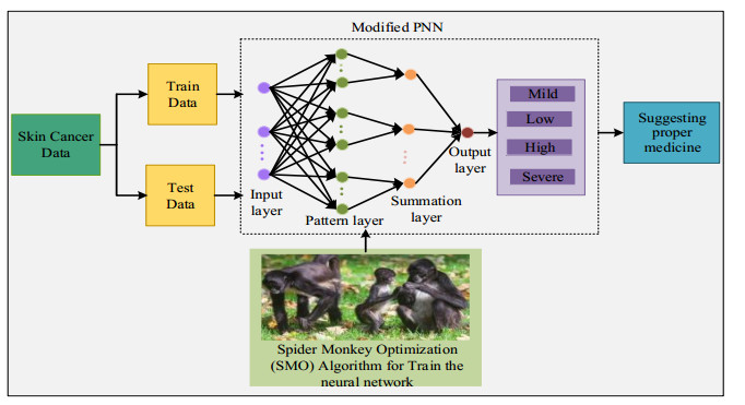
Skin cancer is a pandemic disease now worldwide, and it is responsible for numerous deaths. Early phase detection is pre-eminent for controlling the spread of tumours throughout the body. However, existing algorithms for skin cancer severity detections still have some drawbacks, such as the analysis of skin lesions is not insignificant, slightly worse than that of dermatologists, and costly and time-consuming. Various machine learning algorithms have been used to detect the severity of the disease diagnosis. But it is more complex when detecting the disease. To overcome these issues, a modified Probabilistic Neural Network (MPNN) classifier has been proposed to determine the severity of skin cancer. The proposed method contains two phases such as training and testing the data. The collected features from the data of infected people are used as input to the modified PNN classifier in the current model. The neural network is also trained using Spider Monkey Optimization (SMO) approach. For analyzing the severity level, the classifier predicts four classes. The degree of skin cancer is determined depending on classifications. According to findings, the system achieved a 0.10% False Positive Rate (FPR), 0.03% error and 0.98% accuracy, while previous methods like KNN, NB, RF and SVM have accuracies of 0.90%, 0.70%, 0.803% and 0.86% correspondingly, which is lesser than the proposed approach.
Citation: J. Rajeshwari, M. Sughasiny. Modified PNN classifier for diagnosing skin cancer severity condition using SMO optimization technique[J]. AIMS Electronics and Electrical Engineering, 2023, 7(1): 75-99. doi: 10.3934/electreng.2023005
Skin cancer is a pandemic disease now worldwide, and it is responsible for numerous deaths. Early phase detection is pre-eminent for controlling the spread of tumours throughout the body. However, existing algorithms for skin cancer severity detections still have some drawbacks, such as the analysis of skin lesions is not insignificant, slightly worse than that of dermatologists, and costly and time-consuming. Various machine learning algorithms have been used to detect the severity of the disease diagnosis. But it is more complex when detecting the disease. To overcome these issues, a modified Probabilistic Neural Network (MPNN) classifier has been proposed to determine the severity of skin cancer. The proposed method contains two phases such as training and testing the data. The collected features from the data of infected people are used as input to the modified PNN classifier in the current model. The neural network is also trained using Spider Monkey Optimization (SMO) approach. For analyzing the severity level, the classifier predicts four classes. The degree of skin cancer is determined depending on classifications. According to findings, the system achieved a 0.10% False Positive Rate (FPR), 0.03% error and 0.98% accuracy, while previous methods like KNN, NB, RF and SVM have accuracies of 0.90%, 0.70%, 0.803% and 0.86% correspondingly, which is lesser than the proposed approach.

| [1] |
Putra TA, Rufaida SI and Leu JS (2020) Enhanced skin condition prediction through machine learning using dynamic training and testing augmentation. IEEE Access 8: 40536–40546. https://doi.org/10.1109/ACCESS.2020.2976045 doi: 10.1109/ACCESS.2020.2976045

|
| [2] | Nahata H and Singh SP (2020) Deep learning solutions for skin cancer detection and diagnosis. Machine Learning with Health Care Perspective, 159–182. Springer, Cham. https://doi.org/10.1007/978-3-030-40850-3_8 |
| [3] |
Mijwil MM (2021) Skin cancer disease images classification using deep learning solutions. Multimed Tools Appl 80: 26255–26271. https://doi.org/10.1007/s11042-021-10952-7 doi: 10.1007/s11042-021-10952-7
|
| [4] |
Jeihooni AK and Moradi M (2019) The effect of educational intervention based on PRECEDE model on promoting skin cancer preventive behaviors in high school students. J Cancer Educ 34: 796–802. https://doi.org/10.1007/s13187-018-1376-y doi: 10.1007/s13187-018-1376-y
|
| [5] |
Jeihooni AK and Rakhshani T (2019) The effect of educational intervention based on health belief model and social support on promoting skin cancer preventive behaviors in a sample of Iranian farmers. J Cancer Educ 34: 392–401. https://doi.org/10.1007/s13187-017-1317-1 doi: 10.1007/s13187-017-1317-1
|
| [6] | Mohapatra S, Abhishek NVS, Bardhan D, et al. (2021) Skin cancer classification using convolution neural networks. Advances in Distributed Computing and Machine Learning, 433–442. Springer, Singapore. https://doi.org/10.1007/978-981-15-4218-3_42 |
| [7] |
Maxwell A, Li R, Yang B, et al. (2017) Deep learning architectures for multi-label classification of intelligent health risk prediction. BMC bioinformatics, 18: 121–131. https://doi.org/10.1186/s12859-017-1898-z doi: 10.1186/s12859-017-1898-z
|
| [8] |
Han SS, Park I, Chang SE, et al. (2020) Augmented intelligence dermatology: deep neural networks empower medical professionals in diagnosing skin cancer and predicting treatment options for 134 skin disorders. J Investigat Dermatol 140: 1753–1761. https://doi.org/10.1016/j.jid.2020.01.019 doi: 10.1016/j.jid.2020.01.019
|
| [9] |
Kadampur MA and Riyaee SA (2020) Skin cancer detection: Applying a deep learning based model driven architecture in the cloud for classifying dermal cell images. Informatics in Medicine Unlocked 18: 100282. https://doi.org/10.1016/j.imu.2019.100282 doi: 10.1016/j.imu.2019.100282
|
| [10] | Nahata H and Singh SP (2020) Deep learning solutions for skin cancer detection and diagnosis. Machine Learning with Health Care Perspective, 159–182. Springer, Cham. https://doi.org/10.1007/978-3-030-40850-3_8 |
| [11] |
Pacheco AGC and Krohling A (2020) The impact of patient clinical information on automated skin cancer detection. Comput biol med 116: 103545. https://doi.org/10.1016/j.compbiomed.2019.103545 doi: 10.1016/j.compbiomed.2019.103545
|
| [12] |
Höhn J, Hekler A, Krieghoff-Henning E, et al. (2021) Integrating patient data into skin cancer classification using convolutional neural networks: systematic review. J Med Internet Res 23: e20708. https://doi.org/10.2196/20708 doi: 10.2196/20708
|
| [13] |
Bushehri SF and Zarchi MS (2019) An expert model for self-care problems classification using probabilistic neural network and feature selection approach. Appl Soft Comput 82: 105545. https://doi.org/10.1016/j.asoc.2019.105545 doi: 10.1016/j.asoc.2019.105545
|
| [14] |
Han SS, Park I, Chang SE, et al. (2020) Augmented intelligence dermatology: deep neural networks empower medical professionals in diagnosing skin cancer and predicting treatment options for 134 skin disorders. J Invest Dermatol 140: 1753–1761. https://doi.org/10.1016/j.jid.2020.01.019 doi: 10.1016/j.jid.2020.01.019
|
| [15] |
Kadampur MA and Riyaee SA (2020) Skin cancer detection: Applying a deep learning based model driven architecture in the cloud for classifying dermal cell images. Informatics in Medicine Unlocked 18: 100282. https://doi.org/10.1016/j.imu.2019.100282 doi: 10.1016/j.imu.2019.100282
|
| [16] | Huang CW, Nguyen AP, Wu CC, et al. (2021) Develop a Prediction Model for Nonmelanoma Skin Cancer Using Deep Learning in EHR Data. Soft Computing for Biomedical Applications and Related Topics, 11–18. Springer, Cham. https://doi.org/10.1007/978-3-030-49536-7_2 |
| [17] | Nahata H and Singh S (2020) Deep learning solutions for skin cancer detection and diagnosis. Machine Learning with Health Care Perspective, 2020,159–182. Springer, Cham. https://doi.org/10.1007/978-3-030-40850-3_8 |
| [18] |
Abhishek K, Kawahara J and Hamarneh G (2021) Predicting the clinical management of skin lesions using deep learning. Scientific reports 11: 1–14. https://doi.org/10.1038/s41598-021-87064-7 doi: 10.1038/s41598-021-87064-7
|
| [19] | Ashraf R, Kiran I, Mahmood T, et al. (2020) An efficient technique for skin cancer classification using deep learning. 2020 IEEE 23rd International Multitopic Conference (INMIC), 1–5. IEEE. https://doi.org/10.1109/INMIC50486.2020.9318164 |
| [20] |
Maron RC, Schlager JG, Haggenmüller S, et al. (2021) A benchmark for neural network robustness in skin cancer classification. Eur J Cancer 155: 191–199. https://doi.org/10.1016/j.ejca.2021.06.047 doi: 10.1016/j.ejca.2021.06.047
|
| [21] |
Ali MS, Miah MS, Haque J, et al. (2021) An enhanced technique of skin cancer classification using deep convolutional neural network with transfer learning models. Machine Learning with Applications 5: 100036. https://doi.org/10.1016/j.mlwa.2021.100036 doi: 10.1016/j.mlwa.2021.100036
|
| [22] | Pramanik A and Chakraborty R (2021) A Deep Learning Prediction Model for Detection of Cancerous Lesions from Dermatoscopic Images. Advanced Machine Learning Approaches in Cancer Prognosis, 395–423. Springer, Cham. https: //doi.org/10.1007/978-3-030-71975-3_15 |
| [23] | Salian AC, Vaze S, Singh P, et al. (2020) Skin lesion classification using deep learning architectures. 2020 3rd International conference on communication system, computing and IT applications (CSCITA), 168–173. IEEE. https://doi.org/10.1109/CSCITA47329.2020.9137810 |
| [24] |
Wang JS, Song JD and Gao J (2015) Rough set-probabilistic neural networks fault diagnosis method of polymerization kettle equipment based on shuffled frog leaping algorithm. Information 6: 49–68. https://doi.org/10.3390/info6010049 doi: 10.3390/info6010049
|
| [25] |
Chakravarthy SSR and Rajaguru H (2015) Lung cancer detection using probabilistic neural network with modified crow-search algorithm. Asian Pacific journal of cancer prevention: APJCP 20: 2159. https://doi.org/10.31557/APJCP.2019.20.7.2159 doi: 10.31557/APJCP.2019.20.7.2159
|
| [26] | Sharma H, Hazrati G and Bansal JC (2019) Spider monkey optimization algorithm. Evolutionary and swarm intelligence algorithms, 43–59. Springer, Cham. https://doi.org/10.1007/978-3-319-91341-4_4 |
| [27] |
Kumar S, Sharma B, Sharma VK, et al. (2020) Plant leaf disease identification using exponential spider monkey optimization. Sustainable computing: Informatics and systems 28: 100283. https://doi.org/10.1016/j.suscom.2018.10.004 doi: 10.1016/j.suscom.2018.10.004
|
| [28] |
Rajeshwari J and Sughasiny M (2022) Modified Filter Based Feature Selection Technique for Dermatology Dataset Using Beetle Swarm Optimization. EAI Endorsed Trans S, e2-e2. https://doi.org/10.4108/eetsis.vi.1998 doi: 10.4108/eetsis.vi.1998
|
| [29] |
Rajeshwari J and Sughasiny M (2022) Dermatology disease prediction based on firefly optimization of ANFIS classifier. AIMS Electronics and Electrical Engineering 6: 61–80. https://doi.org/10.3934/electreng.2022005 doi: 10.3934/electreng.2022005
|
| [30] | Dermatology Data set. Available from: https://archive.ics.uci.edu/ml/datasets/dermatology. |
| [31] | Izonin I, Tkachenko R, Ryvak L, et al. (2020) Addressing Medical Diagnostics Issues: Essential Aspects of the PNN-based Approach. IDDM, 209–218. |
| [32] |
Izonin I, Tkachenko R, Gregus M, et al. (2021) Hybrid Classifier via PNN-based Dimensionality Reduction Approach for Biomedical Engineering Task. Procedia Computer Science 191: 230–237. https://doi.org/10.1016/j.procs.2021.07.029 doi: 10.1016/j.procs.2021.07.029
|
| [33] |
Izonin I, Tkachenko R, Gregus M, et al. (2022) PNN-SVM Approach of Ti-Based Powder's Properties Evaluation for Biomedical Implants Production. CMC-COMPUT MATER CON 71: 5933–5947. https://doi.org/10.32604/cmc.2022.022582 doi: 10.32604/cmc.2022.022582
|
| [34] |
Guan Y, Aamir M, Rahman Z, et al. (2021) A framework for efficient brain tumor classification using MRI images. Math Biosci Eng 18: 5790–5815. https://doi.org/10.3934/mbe.2021292 doi: 10.3934/mbe.2021292
|
| [35] |
Aamir M, Rahman Z, Dayo ZA, et al. (2022) A deep learning approach for brain tumor classification using MRI images. Comput Electr Eng 101: 108105. https://doi.org/10.1016/j.compeleceng.2022.108105 doi: 10.1016/j.compeleceng.2022.108105
|


Figures(15) / Tables(4)

J. Rajeshwari, M. Sughasiny. Modified PNN classifier for diagnosing skin cancer severity condition using SMO optimization technique[J]. AIMS Electronics and Electrical Engineering, 2023, 7(1): 75-99. doi: 10.3934/electreng.2023005


 DownLoad: