A novel node selection method for wireless distributed edge storage based on SDN and a maldistributed decision model

Yejin Yang; Miao Ye; Qiuxiang Jiang; Peng Wen; Yejin Yang; Miao Ye; Qiuxiang Jiang; Peng Wen

doi:10.3934/era.2024056

Electronic Research Archive

2024, Volume 32, Issue 2: 1160-1190. doi: 10.3934/era.2024056

Previous Article Next Article

Research article Special Issues

A novel node selection method for wireless distributed edge storage based on SDN and a maldistributed decision model

1.
School of Information and Communications, Guilin University of Electronic Technology, China
2.
Guangxi Key Laboratory of Wireless Wideband Communication and Signal Processing, Guilin University of Electronic Technology, Guilin 541004, China
3.
Ministry of Education Key Laboratory of Cognitive Radio and Information Processing, Guilin University of Electronic Technology, Guilin 541004, China

Received: 26 September 2023 Revised: 20 December 2023 Accepted: 08 January 2024 Published: 29 January 2024

In distributed edge storage, data storage data is allocated to network edge devices to achieve low latency, high security, and flexibility. However, traditional systems for distributed edge storage only consider individual factors, such as node capacity, while overlooking the network status and the load states of the storage nodes, thereby impacting the system's read and write performance. Moreover, these systems exhibit inadequate scalability in widely adopted wireless terminal application scenarios. To overcome these challenges, this paper introduces a software-defined edge storage model and a distributed edge storage architecture grounded in software-defined networking (SDN) and the Server Message Block (SMB) protocol. A data storage node selection and distribution algorithm is formulated based on a maldistributed decision model that comprehensively considers the network and storage node load states. A system prototype is implemented in combination with 5G wireless communication technology. The experimental results demonstrate that, in comparison to conventional distributed edge storage systems, the proposed wireless distributed edge storage system exhibits significantly enhanced performance under high load conditions, demonstrating superior scalability and adaptability. This approach effectively addresses the scalability limitation, rendering it suitable for edge scenarios in mobile applications and reducing hardware deployment costs.
- distributed edge storage,
- software-defined networking,
- node selection algorithm,
- 5G wireless communication
Citation: Yejin Yang, Miao Ye, Qiuxiang Jiang, Peng Wen. A novel node selection method for wireless distributed edge storage based on SDN and a maldistributed decision model[J]. Electronic Research Archive, 2024, 32(2): 1160-1190. doi: 10.3934/era.2024056

Related Papers:

Abstract

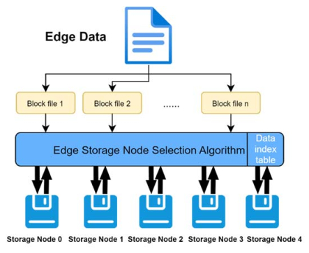
In distributed edge storage, data storage data is allocated to network edge devices to achieve low latency, high security, and flexibility. However, traditional systems for distributed edge storage only consider individual factors, such as node capacity, while overlooking the network status and the load states of the storage nodes, thereby impacting the system's read and write performance. Moreover, these systems exhibit inadequate scalability in widely adopted wireless terminal application scenarios. To overcome these challenges, this paper introduces a software-defined edge storage model and a distributed edge storage architecture grounded in software-defined networking (SDN) and the Server Message Block (SMB) protocol. A data storage node selection and distribution algorithm is formulated based on a maldistributed decision model that comprehensively considers the network and storage node load states. A system prototype is implemented in combination with 5G wireless communication technology. The experimental results demonstrate that, in comparison to conventional distributed edge storage systems, the proposed wireless distributed edge storage system exhibits significantly enhanced performance under high load conditions, demonstrating superior scalability and adaptability. This approach effectively addresses the scalability limitation, rendering it suitable for edge scenarios in mobile applications and reducing hardware deployment costs.

References

[1]	K. Cao, Y. Liu, G. Meng, Q. Sun, An overview on edge computing research, IEEE Access, 8 (2020), 85714–85728. https://doi.org/10.1109/ACCESS.2020.2991734 doi: 10.1109/ACCESS.2020.2991734
[2]	J. Xia, G. Cheng, S. Gu, D. Guo, Secure and trust-oriented edge storage for Internet of Things, IEEE Internet Things J., 7 (2019), 4049–4060. https://doi.org/10.1109/JIOT.2019.2962070 doi: 10.1109/JIOT.2019.2962070
[3]	M. U. A. Siddiqui, F. Qamar, M. Tayyab, M. N. Hindia, Q. N. Nguyen, R. Hassan, Mobility management issues and solutions in 5G-and-beyond networks: a comprehensive review, Electronics, 11 (2022), 1366. https://doi.org/10.3390/electronics11091366 doi: 10.3390/electronics11091366
[4]	P. Yang, N. Xiong, J. Ren, Data security and privacy protection for cloud storage: A survey, IEEE Access, 8 (2020), 131723–131740. https://doi.org/10.1109/ACCESS.2020.3009876 doi: 10.1109/ACCESS.2020.3009876
[5]	J. Wu, Y. Li, F. Ren, B. Yang, Robust and auditable distributed data storage with scalability in edge computing, Ad Hoc Networks, 117 (2021), 102494. https://doi.org/10.1016/j.adhoc.2021.102494 doi: 10.1016/j.adhoc.2021.102494
[6]	M. Legault, A practitioner's view on distributed storage systems: Overview, challenges and potential solutions, Technol. Innovation Manage. Rev., 11 (2021), 32–41. https://doi.org/10.22215/timreview/1448 doi: 10.22215/timreview/1448
[7]	W. Liu, Research on cloud computing security problem and strategy, in 2012 2nd International Conference on Consumer Electronics, Communications and Networks (CECNet), 8 (2012), 1216–1219. https://doi.org/10.1109/CECNet.2012.6202020
[8]	G. Zhu, D. Liu, Y. Du, C. You, J. Zhang, K. Huang, Toward an intelligent edge: Wireless communication meets machine learning, IEEE Commun. Mag., 58 (2020), 19–25. https://doi.org/10.1109/MCOM.001.1900103 doi: 10.1109/MCOM.001.1900103
[9]	J. Thompson, X. Ge, H. C. Wu, R. Irmer, H. Jiang, G. Fettweis, et al., 5G wireless communication systems: Prospects and challenges, IEEE Commun. Mag., 52 (2014), 62–64. https://doi.org/10.1109/MCOM.2014.6736744 doi: 10.1109/MCOM.2014.6736744
[10]	W. Li, Q. Li, L. Chen, F. Wu, J. Ren, A storage resource collaboration model among edge nodes in edge federation service, IEEE Trans. Veh. Technol., 71 (2022), 9212–9224. https://doi.org/10.1109/TVT.2022.3179363 doi: 10.1109/TVT.2022.3179363
[11]	C. Roy, S. Misra, J. Maiti, M. S. Obaidat, DENSE: Dynamic edge node selection for safety-as-a-service, in 2019 IEEE Global Communications Conference (GLOBECOM), 23 (2019), 1–6. https://doi.org/10.1109/globecom38437.2019.9014180
[12]	M. Abd-El-Malek, W. V. Courtright Ⅱ, C. Cranor, G. R. Ganger, J. Hendricks, A. J. Klosterman, et al., Ursa minor: Versatile cluster-based storage, FAST, 5 (2005), 5.
[13]	D. Puthal, R. Ranjan, A. Nanda, P. Nanda, P. P. Jayaraman, A. Y. Zomaya, Secure authentication and load balancing of distributed edge datacenters, J. Parallel Distrib. Comput., 124 (2019), 60–69. https://doi.org/10.1016/j.jpdc.2018.10.007 doi: 10.1016/j.jpdc.2018.10.007
[14]	Y. Zhang, S. Debroy, P. Calyam, Network measurement recommendations for performance bottleneck correlation analysis, in 2016 IEEE International Symposium on Local and Metropolitan Area Networks (LANMAN), 12 (2016), 1–7.
[15]	R. G. Clegg, M. S. Withall, A. W. Moore, I. W. Phillips, D. J. Parish, M. Rio, et al., Challenges in the capture and dissemination of measurements from high-speed networks, IET Commun., 3 (2009), 957–966. https://doi.org/10.1049/iet-com.2008.0068 doi: 10.1049/iet-com.2008.0068
[16]	S. E. Engineer, A. Engineer, Structure and Interpretation of the SMB Protocol, Springer, 2018.
[17]	K. Kirkpatrick, Software-defined networking, Commun. ACM, 56 (2013), 16–19. https://doi.org/10.1109/sta.2019.8717234 doi: 10.1109/sta.2019.8717234
[18]	T. D. Nadeau, K. Gray, SDN: Software Defined Networks: An Authoritative Review of Network Programmability Technologies, O'Reilly Media, Inc., 2013.
[19]	M. T. Rashid, D. Zhang, D. Wang, Edgestore: Towards an edge-based distributed storage system for emergency response, in 2019 IEEE 21st International Conference on High Performance Computing and Communications, 31 (2019), 2543–2550. https://doi.org/10.1109/HPCC/SmartCity/DSS.2019.00356
[20]	A. Makris, E. Psomakelis, T. Theodoropoulos, K. Tserpes, Towards a distributed storage framework for edge computing infrastructures, in Proceedings of the 2nd Workshop on Flexible Resource and Application Management on the Edge, 54 (2022), 9–14. https://doi.org/10.1145/3526059.3533617
[21]	K. Sonbol, Ö. Özkasap, I. Al-Oqily, M. Aloqaily, EdgeKV: Decentralized, scalable, and consistent storage for the edge, J. Parallel Distrib. Comput., 144 (2020), 28–40. https://doi.org/10.1016/j.jpdc.2020.05.009 doi: 10.1016/j.jpdc.2020.05.009
[22]	J. Xing, H. Dai, Z. Yu, A distributed multi-level model with dynamic replacement for the storage of smart edge computing, J. Syst. Archit., 83 (2018), 1–11. https://doi.org/10.1016/j.sysarc.2017.11.002 doi: 10.1016/j.sysarc.2017.11.002
[23]	F. Qiao, J. Wu, J. Li, A. K. Bashir, S. Mumtaz, U. Tariq, Trustworthy edge storage orchestration in intelligent transportation systems using reinforcement learning, IEEE Trans. Intell. Transp. Syst., 22 (2020), 4443–4456. https://doi.org/10.1109/TITS.2020.3003211 doi: 10.1109/TITS.2020.3003211
[24]	W. Li, J. Ji, L. Huang, L. Zhang, Global dynamics and control of malicious signal transmission in wireless sensor networks, Nonlinear Anal. Hybrid Syst., 48 (2023), 101324. https://doi.org/10.1016/j.nahs.2022.101324 doi: 10.1016/j.nahs.2022.101324
[25]	W. Li, J. Ji, L. Huang, Z. Cai, Periodic orbit analysis for a delayed model of malicious signal transmission in wireless sensor networks with discontinuous control, Math. Methods Appl. Sci., 46 (2023), 5267–5285. https://doi.org/10.1002/mma.8831 doi: 10.1002/mma.8831
[26]	K. Kontodimas, P. Soumplis, A. Kretsis, P. Kokkinos, E. Varvarigos, Secure distributed storage on cloud-edge infrastructures, in 2021 IEEE 10th International Conference on Cloud Networking, 93 (2021), 127–132. https://doi.org/10.1109/CloudNet53349.2021.9657156
[27]	C. Wu, Y. Chen, Z. Qi, H. Guan, DSPR: Secure decentralized storage with proof-of-replication for edge devices, J. Syst. Archit., 125 (2022), 102441. https://doi.org/10.1016/j.sysarc.2022.102441 doi: 10.1016/j.sysarc.2022.102441
[28]	S. Li, T. Lan, HotDedup: Managing hot data storage at network edge through optimal distributed deduplication, in IEEE INFOCOM 2020-IEEE Conference on Computer Communications, 144 (2020), 247–256. https://doi.org/10.1109/infocom41043.2020.9155233
[29]	K. He, E. Rozner, K. Agarwal, W. Felter, J. Carter, A. Akella, Presto: Edge-based load balancing for fast datacenter networks, ACM SIGCOMM Comput. Commun. Rev., 45 (2015), 465–478. https://doi.org/10.1145/2785956.2787507 doi: 10.1145/2785956.2787507
[30]	C. Hunt, TCP/IP Network Administration, O'Reilly Media, Inc., 2002.
[31]	R. Sharpe, Just what is SMB?, Oct, 8 (2002), 9.
[32]	S. Khan, A. Gani, A. W. A. Wahab, M. Guizani, M. K. Khan, Topology discovery in software defined networks: Threats, taxonomy, and state-of-the-art, IEEE Commun. Surv. Tutorials, 19 (2016), 303–324. https://doi.org/10.1109/COMST.2016.2597193 doi: 10.1109/COMST.2016.2597193
[33]	A. Bianco, R. Birke, L. Giraudo, M. Palacin, Openflow switching: Data plane performance, in 2010 IEEE International Conference on Communications, 18 (2010), 1–5.
[34]	A. Jalili, H. Nazari, S. Namvarasl, M. Keshtgari, A comprehensive analysis on control plane deployment in SDN: In-band versus out-of-band solutions, in 2017 IEEE 4th International Conference on Knowledge-Based Engineering and Innovation (KBEI), 89 (2017), 1025–1031. https://doi.org/10.1109/KBEI.2017.8324949
[35]	F. Hu, Q. Hao, K. Bao, A survey on software-defined network and openflow: From concept to implementation, IEEE Commun. Surv. Tutorials, 16 (2014), 2181–2206. https://doi.org/10.1109/COMST.2014.2326417 doi: 10.1109/COMST.2014.2326417
[36]	M. Noto, H. Sato, A method for the shortest path search by extended Dijkstra algorithm, in SMC 2000 Conference Proceedings. 2000 IEEE International Conference on Systems, Man and Cybernetics, 3 (2000), 2316–2320. https://doi.org/10.1109/ICSMC.2000.886462
[37]	S. Syamsudin, R. Rahim, Study approach technique for order of preference by similarity to ideal solution (TOPSIS), Int. J. Recent Trends Eng. Res., 3 (2017), 268–285.
[38]	R. Rohith, M. Moharir, G. Shobha, SCAPY-A powerful interactive packet manipulation program, in 2018 International Conference on Networking, Embedded and Wireless Systems (ICNEWS), 52 (2018), 1–5. https://doi.org/10.1109/ICNEWS.2018.8903954
[39]	C. E. Palazzi, M. Brunati, M. Roccetti, An OpenWRT solution for future wireless homes, in 2010 IEEE International Conference on Multimedia and Expo, 74 (2010), 1701–1706. https://doi.org/10.1109/ICME.2010.5583223
[40]	B. Pfaff, J. Pettit, T. Koponen, E. Jackson, A. Zhou, J. Rajahalme, et al., The design and implementation of open vSwitch, in 12th USENIX Symposium on Networked Systems Design and Implementation (NSDI 15), 261 (2015), 117–130.
[41]	W. Donat, W. Donat, Introducing the Raspberry Pi, in Learn Raspberry Pi Programming with Python: Learn to Program on the World's Most Popular Tiny Computer, 16 (2018), 1–26.
[42]	S. Vidya, R. Bhaskaran, ARP storm detection and prevention measures, Int. J. Comput. Sci. Issues, 8 (2011), 456.
[43]	V. Rajaravivarma, Virtual local area network technology and applications, in Proceedings the Twenty-Ninth Southeastern Symposium on System Theory, 18 (1997), 49–52. https://doi.org/10.1109/SSST.1997.581577
[44]	W. Li, J. Ji, L. Huang, Global dynamics analysis of a water hyacinth fish ecological system under impulsive control, J. Franklin Inst., 359 (2022), 10628–10652. https://doi.org/10.1016/j.jfranklin.2022.09.030 doi: 10.1016/j.jfranklin.2022.09.030
[45]	A. Tridgell, Samba protocol, Available from: https://www.samba.org/.

Reader Comments

Your name:*

Email:*
© 2024 the Author(s), licensee AIMS Press. This is an open access article distributed under the terms of the Creative Commons Attribution License (http://creativecommons.org/licenses/by/4.0)