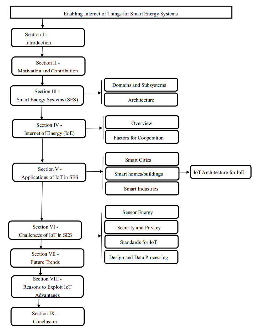
Internet of Things for smart energy systems: A review on its applications, challenges and future trends

Efe Francis Orumwense; Khaled Abo-Al-Ez; Efe Francis Orumwense; Khaled Abo-Al-Ez

doi:10.3934/electreng.2023004

AIMS Electronics and Electrical Engineering

2023, Volume 7, Issue 1: 50-74. doi: 10.3934/electreng.2023004

Previous Article Next Article

Review

Internet of Things for smart energy systems: A review on its applications, challenges and future trends

Centre for Distributed Power and Electronic Research, Cape Peninsula University of Technology, PO Box 1906, 7530, Bellville, Cape Town, South Africa

Received: 31 August 2022 Revised: 05 November 2022 Accepted: 27 November 2022 Published: 20 December 2022

Internet of Things (IoT) is a terminology used for a mixed connection of heterogeneous objects to the internet and to each other with the employment of recent technological and communication infrastructures. Its incorporation into engineering systems have gradually become very popular in recent times as it promises to transform and ease the life of end users. The use of IoT in smart energy systems (SES) facilitates an ample offer of variety of applications that transverses through a wide range of areas in energy systems. With the numerous benefits that includes unmatched fast communication between subsystems, the maximization of energy use, the decrease in environmental impacts and a boost in the dividends of renewable energies, IoT has grown into an emerging innovative technology to be integrated into smart energy systems. In this work, we have provided an overview of the link between SES, IoT and Internet of Energy (IoE). The main applications of IoT in smart energy systems consisting of smart industries, smart homes and buildings, and smart cities are explored and analyzed. The paper also explores the challenges limiting the employment of IoT technologies in SES and the possible remedies to these challenges. In addition, the future trends of this technology, its research direction and reasons why industry should adopt it are also addressed. The aim of this work is to furnish researchers in this field, decision and energy policy makers, energy economist and energy administrators with a possible literature outline on the roles and impacts of IoT technology in smart energy systems.

Keywords:

Citation: Efe Francis Orumwense, Khaled Abo-Al-Ez. Internet of Things for smart energy systems: A review on its applications, challenges and future trends[J]. AIMS Electronics and Electrical Engineering, 2023, 7(1): 50-74. doi: 10.3934/electreng.2023004

Related Papers:

[1]	Kun-Peng Jin, Can Liu . RETRACTED ARTICLE: Decay estimates for the wave equation with partial boundary memory damping. Networks and Heterogeneous Media, 2024, 19(3): 1402-1423. doi: 10.3934/nhm.2024060
[2]	Yaru Xie, Genqi Xu . The exponential decay rate of generic tree of 1-d wave equations with boundary feedback controls. Networks and Heterogeneous Media, 2016, 11(3): 527-543. doi: 10.3934/nhm.2016008
[3]	Ye Sun, Daniel B. Work . Error bounds for Kalman filters on traffic networks. Networks and Heterogeneous Media, 2018, 13(2): 261-295. doi: 10.3934/nhm.2018012
[4]	Zhong-Jie Han, Enrique Zuazua . Decay rates for $1-d$ heat-wave planar networks. Networks and Heterogeneous Media, 2016, 11(4): 655-692. doi: 10.3934/nhm.2016013
[5]	Abdelaziz Soufyane, Adel M. Al-Mahdi, Mohammad M. Al-Gharabli, Imad Kissami, Mostafa Zahri . Stability results of a swelling porous-elastic system with two nonlinear variable exponent damping. Networks and Heterogeneous Media, 2024, 19(1): 430-455. doi: 10.3934/nhm.2024019
[6]	Clinton Innes, Razvan C. Fetecau, Ralf W. Wittenberg . Modelling heterogeneity and an open-mindedness social norm in opinion dynamics. Networks and Heterogeneous Media, 2017, 12(1): 59-92. doi: 10.3934/nhm.2017003
[7]	Serge Nicaise, Julie Valein . Stabilization of the wave equation on 1-d networks with a delay term in the nodal feedbacks. Networks and Heterogeneous Media, 2007, 2(3): 425-479. doi: 10.3934/nhm.2007.2.425
[8]	Gildas Besançon, Didier Georges, Zohra Benayache . Towards nonlinear delay-based control for convection-like distributed systems: The example of water flow control in open channel systems. Networks and Heterogeneous Media, 2009, 4(2): 211-221. doi: 10.3934/nhm.2009.4.211
[9]	Linglong Du . Long time behavior for the visco-elastic damped wave equation in $\mathbb{R}^n_+$ and the boundary effect. Networks and Heterogeneous Media, 2018, 13(4): 549-565. doi: 10.3934/nhm.2018025
[10]	Yacine Chitour, Guilherme Mazanti, Mario Sigalotti . Stability of non-autonomous difference equations with applications to transport and wave propagation on networks. Networks and Heterogeneous Media, 2016, 11(4): 563-601. doi: 10.3934/nhm.2016010

Abstract

The journal retracts the paper entitled "Decay estimates for the wave equation with partial boundary memory damping" ^[1].

After the article was published, the authors decided to withdraw the article.

This retraction was approved by the Editor in Chief of the journal Networks and Heterogeneous Media.

References

[1]	International Energy Agency (IEA), 2022. Global Energy & CO2 Status Report 2022.
[2]	IEA, 2019. Global Energy and CO2 Report 2019. Available from: https://iea.org/reports/global-energy-co2-status-report-2019
[3]	Jensen M (1993) The Modern Industrial Revolution, Exit, and the Failure of Internal Control Systems. J Financ 48: 831–880. https://doi.org/10.1111/j.1540-6261.1993.tb04022.x doi: 10.1111/j.1540-6261.1993.tb04022.x
[4]	Saleem Y, Crespi N, Rehmani MH, et al. (2017) Internet of things-aided Smart Grid: technologies, architectures, applications, prototypes, and future research directions. IEEE Access 7: 62962-63003. https://doi.org/10.1109/ACCESS.2019.2913984. doi: 10.1109/ACCESS.2019.2913984
[5]	Chelloug SA, El-Zawawy MA (2017) Middleware for Internet of Things: Survey and Challenges. Intell Autom Soft Comput 3: 70–95. https://doi.org/10.1080/10798587.2017.1290328 doi: 10.1080/10798587.2017.1290328
[6]	Shrouf F, Ordieres J, Miragliotta G (2014) Smart factories in Industry 4.0: A review of the concept and of energy management approached in production based on the Internet of Things paradigm. Proceedings of the 2014 IEEE International Conference on Industrial Engineering and Engineering Management; 697–701. https://doi.org/10.1109/IEEM.2014.7058728
[7]	Wang Q, Wang YG (2018) Research on Power Internet of Things Architecture for Smart Grid Demand. 2018 2nd IEEE Conference on Energy Internet and Energy System Integration (EI2). https://doi.org/10.1109/EI2.2018.8582132
[8]	Vu TL, Le NT, Jang YM, et al. (2018) An Overview of Internet of Energy (IoE) Based Building Energy Management System. 2018 International Conference on Information and Communication Technology Convergence (ICTC), 852-855. https://doi.org/10.1109/ICTC.2018.8539513
[9]	Bin X, Qing C, Jun M, et al. (2019) Research on a Kind of Ubiquitous Power Internet of Things System for Strong Smart Power Grid. 2019 IEEE Innovative Smart Grid Technologies - Asia (ISGT Asia), 2805-2808. https://doi.org/10.1109/ISGT-Asia.2019.8881652
[10]	Wang W, Zhou Z (2020) Exploring Novel Internet-of-things Based on Free Space Optical Communications for Smart Grids. 2020 IEEE 4th Conference on Energy Internet and Energy System Integration (EI2), 4277-4281. https://doi.org/10.1109/EI250167.2020.9347166
[11]	Xiang W, Wang Y, Gao X, et al. (2021) Design and Implementation of Internet of Things System Based on Customer Electricity Behavior Analysis. 2021 IEEE 5th Conference on Energy Internet and Energy System Integration (EI2), 3411-3415. https://doi.org/10.1109/EI252483.2021.9713593
[12]	Amin SM, Wollenberg BF (2005) Toward a smart grid: power delivery for the 21st century. IEEE power and energy magazine 3: 34–41. https://doi.org/10.1109/MPAE.2005.1507024 doi: 10.1109/MPAE.2005.1507024
[13]	Orumwense EF, Abo-Al-Ez KM (2019) A systematic review to aligning research paths: Energy cyber-physical systems. Cogent Eng 6: 1700738. https://doi.org/10.1080/23311916.2019.1700738 doi: 10.1080/23311916.2019.1700738
[14]	Zeng Z, Ding T, Xu Y, et al. (2020) Reliability Evaluation for Integrated Power-Gas Systems with Power-to-Gas and Gas Storagesin. IEEE T Power Syst 35: 571-583. https://doi.org/10.1109/TPWRS.2019.2935771 doi: 10.1109/TPWRS.2019.2935771
[15]	Gahleitner G (2013) Hydrogen from renewable electricity: An international review of power-to-gas pilot plants for stationary applications. Int J Hydrogen Energy 38: 2039–2061. https://doi.org/10.1016/j.ijhydene.2012.12.010 doi: 10.1016/j.ijhydene.2012.12.010
[16]	Cui S, Wang Y, Xiao J (2019) Peer-to-Peer Energy Sharing Among Smart Energy Buildings by Distributed Transaction. IEEE T Smart Grid 10: 6491-6501. https://doi.org/10.1109/TSG.2019.2906059 doi: 10.1109/TSG.2019.2906059
[17]	Vision of Smart Energy – Research, development and Demonstration, Smart Energy Networks.
[18]	IEEE smart grid domains - IEEE smart grid. (2020) https://smartgrid.ieee.org/domains.
[19]	Mohassel R, Fung A, Mohammadi F, et al. (2014) A survey of Advanced Metering Infrastructure. International Journal of Electrical Power and Energy Systems 63: 473-484. https://doi.org/10.1016/j.ijepes.2014.06.025 doi: 10.1016/j.ijepes.2014.06.025
[20]	Pereira R, Figueiredo J, Melicio R, et al. (2015) Consumer energy management system with integration of smart meters. Energy Rep 1: 22–29. https://doi.org/10.1016/j.egyr.2014.10.001 doi: 10.1016/j.egyr.2014.10.001
[21]	Sayed K, Gabbar HA (2017) SCADA and smart energy grid control automation. Smart Energy Grid Engineering, 481–514. https://doi.org/10.1016/B978-0-12-805343-0.00018-8
[22]	Mohanty SP, Choppali U, Kougianos K (2016) Everything you wanted to know about smart cities. IEEE Consum Electron Mag 5: 60–70. https://doi.org/10.1109/MCE.2016.2556879 doi: 10.1109/MCE.2016.2556879
[23]	Bouzid AM, Guerrero JM, Cheriti A, et al. (2015) A survey on control of electric power distributed generation systems for microgrid applications. Renew Sustain Energy Rev 44: 751–766. https://doi.org/10.1016/j.rser.2015.01.016 doi: 10.1016/j.rser.2015.01.016
[24]	Haseeb K, Almogren A, Islam N, et al. (2019) An Energy-Efficient and Secure Routing Protocol for Intrusion Avoidance in IoT-Based WSN. Energies 12, 4174. https://doi.org/10.3390/en12214174
[25]	Zouinkhi A, Ayadi H, Val T, et al. (2019) Auto-management of energy in IoT networks. Int J Commun Syst 33: e4168. https://doi.org/10.1002/dac.4168.
[26]	Hö ller J, Tsiatsis V, Mulligan C, et al. (2014) From Machine-to-Machine to the Internet of Things: Introduction to a New Age of Intelligence; Elsevier: Amsterdam, The Netherlands.
[27]	Hersent O, Boswarthick D, Elloumi O (2011) The internet of things: Key Applications and Protocols. John Wiley & Sons. https://doi.org/10.1002/9781119958352
[28]	Tulemissova G (2016) The Impact of the IoT and IoE Technologies on Changes of Knowledge Management Strategy. ECIC2016-Proceedings of the 8th European Conference on Intellectual Capital: ECIC2016, 300. Academic Conferences and publishing limited.
[29]	Zhou K, Yang S, Shao Z (2016) Energy Internet: The business perspective. Appl Energy 178: 212–222. https://doi.org/10.1016/j.apenergy.2016.06.052 doi: 10.1016/j.apenergy.2016.06.052
[30]	Tahanan M, Van Ackooij W, Frangioni A, et al. (2015) Large-scale Unit Commitment under uncertainty. 4OR 13: 115–171, https://doi.org/10.1007/s10288-014-0279-y doi: 10.1007/s10288-014-0279-y
[31]	Anvari-Moghaddam A, Monsef H, Rahimi-Kian A (2015) Cost-effective and comfort-aware residential energy management under different pricing schemes and weather conditions. Energy Build 86: 782–793, https://doi.org/10.1016/j.enbuild.2014.10.017 doi: 10.1016/j.enbuild.2014.10.017
[32]	Mahmud K, Town GE, Morsalin S, et al. (2017) Integration of electric vehicles and management in the internet of energy. Renew Sustain Energy Rev 82: 4179–4203, https://doi.org/10.1016/j.rser.2017.11.004 doi: 10.1016/j.rser.2017.11.004
[33]	Orumwense EF, Abo-Al-Ez K (2019) An Energy Efficient Cognitive Radio based Smart Grid Communication Architecture. Proceedings of the 17^th IEEE Industrial and Commercial Use of Energy, Cape Town, South Africa. https://doi.org/10.2139/ssrn.3638151
[34]	Patil K, Lahudkar PSL (2015) Survey of MAC Layer Issues and Application layer Protocols for Machine-to-Machine Communications. IEEE Internet Things J 2: 175–186. https://doi.org/10.1109/JIOT.2015.2394438 doi: 10.1109/JIOT.2015.2394438
[35]	Li Z, Shahidehpour M, Aminifar F (2017) Cybersecurity in Distributed Power Systems. Proc IEEE, 105: 1367–1388, https://doi.org/10.1109/JPROC.2017.2687865 doi: 10.1109/JPROC.2017.2687865
[36]	Groopman J, Etlinger S (2015) Consumer Perceptions of Privacy in the Internet of Things: What Brands Can Learn from a Concerned Citizenry. Altimeter Group: San Francisco, CA, USA, 1–25.
[37]	Zafar R, Mahmood A, Razzaq S, et al. (2018) Prosumer based energy management and sharing in smart grid. Renew Sustain Energy Rev 82: 1675–1684, https://doi.org/10.1016/j.rser.2017.07.018 doi: 10.1016/j.rser.2017.07.018
[38]	Luna AC, Diaz NL, Graells M, et al. (2016) Cooperative energy management for a cluster of households prosumers. IEEE T Consum Electron 62: 235–242. https://doi.org/10.1109/TCE.2016.7613189 doi: 10.1109/TCE.2016.7613189
[39]	Iannello F, Simeone O, Spagnolini U (2010) Energy Management Policies for Passive RFID Sensors with RF-Energy Harvesting. Proceedings of the 2010 IEEE International Conference on Communications, 1–6, https://doi.org/10.1109/ICC.2010.5502035
[40]	Ramamurthy A, Jain P (2017) The Internet of Things in the Power Sector: Opportunities in Asia and the Pacific. https://doi.org/10.22617/WPS178914-2
[41]	Sigfox, Inc. Utilities & Energy (2019) Available from: https://www.sigfox.com/en/utilities-energy/.
[42]	Immelt JR (2015) The Future of Electricity Is Digital; Technical Report; General Electric: Boston, MA, USA, 2015.
[43]	Huneria HK, Yadav P, Shaw RN, et al. (2021) AI and IOT-Based Model for Photovoltaic Power Generation. Innovations in Electrical and Electronic Engineering, 697-706. https://doi.org/10.1007/978-981-16-0749-3_55
[44]	Singh R, Akram SV, Gehlot A, et al. (2022) Energy System 4.0: Digitalization of the Energy Sector with Inclination towards Sustainability. Sensors 22: 6619. https://doi.org/10.3390/s22176619
[45]	Ejaz W, Naeem M, Shahid A, et al. (2017) Efficient energy management for the internet of things in smart cities. IEEE Commun Mag 55: 84–91. https://doi.org/10.1109/MCOM.2017.1600218CM doi: 10.1109/MCOM.2017.1600218CM
[46]	Mitchell S, Villa N, Stewart-Weeks M, et al. (2013) The Internet of Everything for Cities; Cisco: San Jose, CA, USA, 2013.
[47]	Idwan S, Mahmood I, Zubairi J, et al. (2020) Optimal Management of Solid Waste in Smart Cities using Internet of Things. Wireless Pers Commun 110: 485-501. https://doi.org/10.1007/s11277-019-06738-8 doi: 10.1007/s11277-019-06738-8
[48]	Vakiloroaya V, Samali B, Fakhar A, et al. (2014) A review of different strategies for HVAC energy saving. Energy Convers Manag 77: 738–754. https://doi.org/10.1016/j.enconman.2013.10.023 doi: 10.1016/j.enconman.2013.10.023
[49]	Arasteh H, Hosseinnezhad V, Loia V, et al. (2016) IoT-based smart cities: A survey. Proceedings of the 2016 IEEE 16th International Conference on Environment and Electrical Engineering (EEEIC), 1–6. https://doi.org/10.1109/EEEIC.2016.7555867
[50]	Lee C, Zhang S (2016) Development of an Industrial Internet of Things Suite for Smart Factory towards Re-industrialization in Hong Kong. Proceedings of the 6th International Workshop of Advanced Manufacturing and Automation, 285-289. https://doi.org/10.2991/iwama-16.2016.54
[51]	Reinfurt L, Falkenthal M, Breitenbücher U, et al. (2017) Applying IoT Patterns to Smart Factory Systems. Proceedings of the 2017 Advanced Summer School on Service Oriented Computing (Summer SOC), 66.
[52]	Cheng J, Chen W, Tao F, et al. (2018) Industrial IoT in 5G Environment towards Smart Manufacturing. J Ind Inf Integr 10: 10–19. https://doi.org/10.1016/j.jii.2018.04.001 doi: 10.1016/j.jii.2018.04.001
[53]	IoT application areas (2016) https://www.iot-analytics.com/top-10-iot-project-application-areas-q3-2016/.
[54]	Shi W, Xie X, Chu C, et al. (2015) Distributed Optimal Energy Management in Microgrids. IEEE T Smart Grid 6: 1137–1146. https://doi.org/10.1109/TSG.2014.2373150 doi: 10.1109/TSG.2014.2373150
[55]	Kamalinejad P, Mahapatra C, Sheng Z, et al. (2015) Wireless energy harvesting for the Internet of Things. IEEE Commun Mag 53: 102–108. https://doi.org/10.1109/MCOM.2015.7120024 doi: 10.1109/MCOM.2015.7120024
[56]	Song T, Li R, Mei B, et al. (2017) A privacy preserving communication protocol for IoT applications in smart homes. IEEE Internet Things J 4: 1844–1852. https://doi.org/10.1109/JIOT.2017.2707489. doi: 10.1109/JIOT.2017.2707489
[57]	Fhom HS, Kuntze N, Rudolph C, et al. (2010) A user-centric privacy manager for future energy systems. Proceedings of the 2010 International Conference on Power System Technology, 1–7. https://doi.org/10.1109/POWERCON.2010.5666447.
[58]	Pramudita R, Hariadi IF, Achmad AS (2017) Development of IoT Authentication Mechanisms for Microgrid Applications. 2017 International Symposium on Electronics and Smart Devices (ISESD), 12-17. https://doi.org/10.1109/ISESD.2017.8253297
[59]	Trappe W, Howard R, Moore RS (2015) Low-Energy Security: Limits and Opportunities in the Internet of Things. IEEE Secur Priv 13: 14-21. https://doi.org/10.1109/MSP.2015.7 doi: 10.1109/MSP.2015.7
[60]	IEEE Std 802.15.4-2015 (Revision of IEEE Std 802.15.4-2011) (2016) IEEE Standard for Low-Rate Wireless Networks. IEEE Stand, 1–708, https://doi.org/10.1109/IEEESTD.2016.7460875
[61]	Al-Qaseemi SA, Almulhim HA, Almulhim MF, et al. (2016) IoT architecture challenges and issues: Lack of standardization. Proceedings of the 2016 Future Technologies Conference (FTC), 731–738. https://doi.org/10.1109/FTC.2016.7821686
[62]	Stojmenovic I (2014) Machine-to-Machine Communications with In-Network Data Aggregation, Processing, and Actuation for Large-Scale Cyber-Physical Systems. IEEE Internet Things J 1: 122–128. https://doi.org/10.1109/JIOT.2014.2311693 doi: 10.1109/JIOT.2014.2311693
[63]	Lloret J, Tomas J, Canovas A, et al. (2016) An Integrated IoT Architecture for Smart Metering. IEomEE Commun Mag 54: 50–57. https://doi.org/10.1109/MCOM.2016.1600647CM doi: 10.1109/MCOM.2016.1600647CM
[64]	Breur T (2015) Big data and Internet of Things. J Mark Anal 3: 1–4. https://doi.org/10.1057/jma.2015.7 doi: 10.1057/jma.2015.7
[65]	Shakerighadi B, Anvari-Moghaddam A, Vasquez JC, et al. (2018) Internet of things for modern energy systems: state-of-the-art, challenges, and open issues. Energies 11: 1252. 10.3390/en11051252
[66]	Xu J, Yao J, Wang L, et al. (2017) Narrowband internet of things: evolutions, technologies and open issues. IEEE Internet of things journal 5: 1449-1462. https://doi.org/10.1109/JIOT.2017.2783374 doi: 10.1109/JIOT.2017.2783374
[67]	Venkatesh N (2015) Ensuring Coexistence of IoT Wireless Protocols Using a Convergence Module to Avoid Contention, Embedded Innovator, 12th Edition, 2015.
[68]	Bedi G, Venayagamoorthy GK, Singh R (2016) Navigating the challenges of Internet of Things (IoT) for power and energy systems. 2016 Clemson University Power Systems Conference (PSC). https://doi.org/10.1109/PSC.2016.7462853
[69]	Singh R, Akram SV, Gehlot A, et al. (2022) Energy System 4.0: Digitalization of the Energy Sector with Inclination towards Sustainability. Sensors 22: 6619. https://doi.org/10.3390/s22176619.
[70]	Rana MM, Xiang W, Wang E (2018) IoT-based state estimation for microgrids. IEEE Internet of things Journal 5: 1345-1346. https://doi.org/10.1109/JIOT.2018.2793162 doi: 10.1109/JIOT.2018.2793162
[71]	Rana MM, Xiang W, Wang E, et al. (2017) IoT Infrastructure and Potential Application to Smart Grid Communications. IEEE Global communication conference (GLOBECOM 2017). https://doi.org/10.1109/GLOCOM.2017.8254511
[72]	Naqvi SAR, Hassan SA, Hussain F (2017) IoT Applications and Business Models. Springer Briefs in Electrical and Computer Engineering, 45–61. https://doi.org/10.1007/978-3-319-55405-1_4
[73]	Research and Markets (2020) Global Internet of Things (IoT) in Energy Market Size Expected to Grow from USD 20.2 billion in 2020 to USD 35.2 billion by 2025, at a CAGR of 11.8%. https://www.globenewswire.com/news-release/2020/05/28/2040020/28124/en/Global-Internet-of-Things-IoT-in-Energy-Market-Size-Expected-to-Grow-from-USD-20-2-billion-in-2020-to-USD-35-2-billion-by-2025-at-a-CAGR-of-11-8.html.
[74]	IoT Analytics, January (2022) https://iot-analytics.com/product/list-of1600-enterprise-iot-projects-2022/.
[75]	The Insight planners, July (2022) https://www.theinsightpartners.com/reports/south-africa-iot-market/. Accessed 1o August 2022.
[76]	Growth Enabler (2017) Market pulse report, Internet of Things (IoT). 1–35. GrowthEnabler. https://growthenabler.com/flipbook/pdf/IOTReport.pdf.
[77]	Hawlitschek F, Notheisen B, Teubner T (2018) The limits of trust-free systems: A literature review on blockchain technology and trust in the sharing economy. Electron Commer Res Appl 29: 50–63. https://doi.org/10.1016/j.elerap.2018.03.005 doi: 10.1016/j.elerap.2018.03.005
[78]	Christidis K, Devetsikiotis M (2016) Blockchains and Smart Contracts for the Internet of Things. IEEE Access 4: 2292–2303. https://doi.org/10.1109/ACCESS.2016.2566339. doi: 10.1109/ACCESS.2016.2566339
[79]	LG and Samsung to Show Off New Food Identifying Smart Fridges at CES Next Week: https://thespoon.tech/lg-and-samsung-to-show-off-new-food-identifying-smart-fridges-at-ces-next-week/
[80]	IoT Statistics. https://www.statista.com/statistics/471264/iot-number-of-connected-devices-worldwide/.
[81]	Abalansa S, El Mahrad B, Icely J, et al. (2021) Electronic Waste, an Environmental Problem Exported to Developing Countries: The GOOD, the BAD and the UGLY. Sustainability 13: 5302. https://doi.org/10.3390/su13095302. doi: 10.3390/su13095302
[82]	Zhu C, Leung VCM, Shu L, et al. (2015) Green Internet of Things for Smart World. IEEE Access 3: 2151–2162. https://doi.org/10.1109/ACCESS.2015.2497312. doi: 10.1109/ACCESS.2015.2497312
[83]	Kabalci Y, Ali M (2019) Emerging LPWAN Technologies for Smart Environments: An Outlook. Proceedings of the 2019 1st Global Power, Energy and Communication Conference (GPECOM), 24–29. https://doi.org/10.1109/GPECOM.2019.8778626
[84]	Bembe M, Abu-Mahfouz A, Masonta M, et al. (2019) A survey on low-power wide area networks for IoT applications. Telecommun Syst 71: 249–274. https://doi.org/10.1007/s11235-019-00557-9. doi: 10.1007/s11235-019-00557-9

Reader Comments

Your name:*

Email:*
© 2023 the Author(s), licensee AIMS Press. This is an open access article distributed under the terms of the Creative Commons Attribution License (http://creativecommons.org/licenses/by/4.0)