The rate of increase in skin cancer incidences has become worrying in recent decades. This is because of constraints like eventual draining of ozone levels, air's defensive channel capacity and progressive arrival of Sun-oriented UV radiation to the Earth's surface. The failure to diagnose skin cancer early is one of the leading causes of death from the disease. Manual detection processes consume more time well as not accurate, so the researchers focus on developing an automated disease classification method. In this paper, an automated skin cancer classification is achieved using an adaptive neuro-fuzzy inference system (ANFIS). A hybrid feature selection technique was developed to choose relevant feature subspace from the dermatology dataset. ANFIS analyses the dataset to give an effective outcome. ANFIS acts as both fuzzy and neural network operations. The input is converted into a fuzzy value using the Gaussian membership function. The optimal set of variables for the Membership Function (MF) is generated with the help of the firefly optimization algorithm (FA). FA is a new and strong meta-heuristic algorithm for solving nonlinear problems. The proposed method is designed and validated in the Python tool. The proposed method gives 99% accuracy and a 0.1% false-positive rate. In addition, the proposed method outcome is compared to other existing methods like improved fuzzy model (IFM), fuzzy model (FM), random forest (RF), and Naive Byes (NB).
Citation: J. Rajeshwari, M. Sughasiny. Dermatology disease prediction based on firefly optimization of ANFIS classifier[J]. AIMS Electronics and Electrical Engineering, 2022, 6(1): 61-80. doi: 10.3934/electreng.2022005
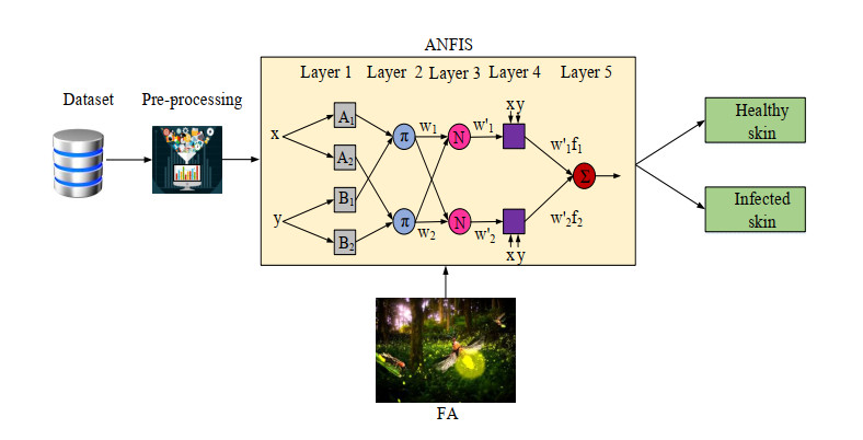
The rate of increase in skin cancer incidences has become worrying in recent decades. This is because of constraints like eventual draining of ozone levels, air's defensive channel capacity and progressive arrival of Sun-oriented UV radiation to the Earth's surface. The failure to diagnose skin cancer early is one of the leading causes of death from the disease. Manual detection processes consume more time well as not accurate, so the researchers focus on developing an automated disease classification method. In this paper, an automated skin cancer classification is achieved using an adaptive neuro-fuzzy inference system (ANFIS). A hybrid feature selection technique was developed to choose relevant feature subspace from the dermatology dataset. ANFIS analyses the dataset to give an effective outcome. ANFIS acts as both fuzzy and neural network operations. The input is converted into a fuzzy value using the Gaussian membership function. The optimal set of variables for the Membership Function (MF) is generated with the help of the firefly optimization algorithm (FA). FA is a new and strong meta-heuristic algorithm for solving nonlinear problems. The proposed method is designed and validated in the Python tool. The proposed method gives 99% accuracy and a 0.1% false-positive rate. In addition, the proposed method outcome is compared to other existing methods like improved fuzzy model (IFM), fuzzy model (FM), random forest (RF), and Naive Byes (NB).

| [1] |
Kadampur MA, Riyaee SA (2020) Skin cancer detection: Applying a deep learning-based model driven architecture in the cloud for classifying dermal cell images. Informatics in Medicine Unlocked 18: 100282. https://doi.org/10.1016/j.imu.2019.100282 doi: 10.1016/j.imu.2019.100282

|
| [2] | Pintelas E, Liaskos M, Livieris IE, et al. (2021) A novel explainable image classification framework: case study on skin cancer and plant disease prediction. Neural Computing and Applications, 1-19. https://doi.org/10.1007/s00521-021-06141-0 |
| [3] |
Magalhaes C, Manuel J, Tavares RS, et al. (2021) Comparison of machine learning strategies for infrared thermography of skin cancer. Biomed Signal Proces 69: 102872. https://doi.org/10.1016/j.bspc.2021.102872 doi: 10.1016/j.bspc.2021.102872
|
| [4] | Das T, Kumar V, Prakash A, Lynn AM (2021) Artificial Intelligence in Skin Cancer: Diagnosis and Therapy. In Skin Cancer: Pathogenesis and Diagnosis, Springer, Singapore, 143-171. https://doi.org/10.1007/978-981-16-0364-8_9 |
| [5] |
Verma, AK, Pal S, Tiwari BB (2020) Skin disease prediction using ensemble methods and a new hybrid feature selection technique. Iran Journal of Computer Science 3(4): 207-216. https://doi.org/10.1007/s42044-020-00058-y doi: 10.1007/s42044-020-00058-y
|
| [6] | Al-Obeidat F, Rocha Á, Akram M, et al. (2021) (CDRGI)-Cancer detection through relevant genes identification. Neural Computing and Applications, 1-8. https://doi.org/10.1007/s00521-021-05739-8 |
| [7] | Ghanshala T, Tripathi V, Pant B (2021) An efficient image-based skin cancer classification framework using neural network. In Research in Intelligent and Computing in Engineering, Springer, Singapore, 851-858. https://doi.org/10.1007/978-981-15-7527-3_81 |
| [8] |
Chaturvedi SS, Tembhurne JV, Diwan T (2020) A multi-class skin Cancer classification using deep convolutional neural networks. Multimed Tools Appl 79: 28477-28498. https://doi.org/10.1007/s11042-020-09388-2 doi: 10.1007/s11042-020-09388-2
|
| [9] | Myakinin OO, Khramov AG, Raupov DS, et al. (2020) Texture Analysis in Skin Cancer Tumor Imaging. In Multimodal Optical Diagnostics of Cancer, Springer, Cham, 465-504. https://doi.org/10.1007/978-3-030-44594-2_13 |
| [10] |
Weli ZNS (2020) Data Mining in Cancer Diagnosis and Prediction: Review about Latest Ten Years. Current Journal of Applied Science and Technology 39: 11-32. https://doi.org/10.9734/cjast/2020/v39i630555 doi: 10.9734/cjast/2020/v39i630555
|
| [11] |
Wang Y, Louie DC, Cai J, et al. (2021) Deep learning enhances polarization speckle for in vivo skin cancer detection. Opt Laser Technol 140: 107006. https://doi.org/10.1016/j.optlastec.2021.107006 doi: 10.1016/j.optlastec.2021.107006
|
| [12] |
Thomas SM, Lefevre JG, Baxter G, et al. (2021) Interpretable deep learning systems for multi-class segmentation and classification of non-melanoma skin cancer. Med Image Anal 68: 101915. https://doi.org/10.1016/j.media.2020.101915 doi: 10.1016/j.media.2020.101915
|
| [13] |
Mohan S, Thirumalai C, Srivastava G (2019) Effective heart disease prediction using hybrid machine learning techniques. IEEE access 7: 81542-81554. https://doi.org/10.1109/ACCESS.2019.2923707 doi: 10.1109/ACCESS.2019.2923707
|
| [14] |
Harimoorthy K, Thangavelu M (2021) Multi-disease prediction model using improved SVM-radial bias technique in healthcare monitoring system. J Amb Intel Hum Comp 12: 3715-3723. https://doi.org/10.1007/s12652-019-01652-0 doi: 10.1007/s12652-019-01652-0
|
| [15] |
Ramani R, Devi KV, Soundar KR (2020).MapReduce-based big data framework using modified artificial neural network classifier for diabetic chronic disease prediction. Soft Comput 24: 16335-16345. https://doi.org/10.1007/s00500-020-04943-3 doi: 10.1007/s00500-020-04943-3
|
| [16] |
Dulhare UN (2018) Prediction system for heart disease using Naive Bayes and particle swarm optimization. Biomedical Research 29: 2646-2649. https://doi.org/10.4066/biomedicalresearch.29-18-620 doi: 10.4066/biomedicalresearch.29-18-620
|
| [17] | Dhivyaa CR, Sangeetha K, Balamurugan M, et al. (2020) Skin lesion classification using decision trees and random forest algorithms. J Amb Intel Hum Comp, 1-13. https://doi.org/10.1007/s12652-020-02675-8 |
| [18] |
Petković D, Barjaktarovic M, Milošević S, et al. (2021) Neuro fuzzy estimation of the most influential parameters for Kusum biodiesel performance. Energy 229: 120621. https://doi.org/10.1016/j.energy.2021.120621 doi: 10.1016/j.energy.2021.120621
|
| [19] |
Stojanović J, Petkovic D, Alarifi IM, et al. (2021) Application of distance learning in mathematics through adaptive neuro-fuzzy learning method. Computer Electr Eng 93: 107270. https://doi.org/10.1016/j.compeleceng.2021.107270 doi: 10.1016/j.compeleceng.2021.107270
|
| [20] |
Kuzman B, Petković B, Denić N, et al. (2021) Estimation of optimal fertilizers for optimal crop yield by adaptive neuro fuzzy logic. Rhizosphere 18: 100358. https://doi.org/10.1016/j.rhisph.2021.100358 doi: 10.1016/j.rhisph.2021.100358
|
| [21] | Milić M, Petković B, Selmi A, et al. (2021) Computational evaluation of microalgae biomass conversion to biodiesel. Biomass Convers Bior, 1-8. https://doi.org/10.1007/s13399-021-01314-2 |
| [22] | Lakovic N, Khan A, Petković B, et al. (2021) Management of higher heating value sensitivity of biomass by hybrid learning technique. Biomass Convers Bior, 1-8. https://doi.org/10.1007/s13399-020-01223-w |
| [23] | Petkovic D, Petković B, Kuzman B (2020) Appraisal of information system for evaluation of kinetic parameters of biomass oxidation. Biomass Convers Bior, 1-9. https://doi.org/10.1007/s13399-020-01014-3 |
| [24] |
Gavrilović S, Denić N, Petković D, et al. (2018) Statistical evaluation of mathematics lecture performances by soft computing approach. Comput Appl Eng Educ 26: 902-905. https://doi.org/10.1002/cae.21931 doi: 10.1002/cae.21931
|
| [25] |
Nikolić V, Petković D, Lazov L, et al. (2016) Selection of the most influential factors on the water-jet assisted underwater laser process by adaptive neuro-fuzzy technique. Infrared Phys Techn 77: 45-50. https://doi.org/10.1016/j.infrared.2016.05.021 doi: 10.1016/j.infrared.2016.05.021
|
| [26] |
Milovančević M, Nikolić V, Petkovic D, et al. (2018) Vibration analyzing in horizontal pumping aggregate by soft computing. Measurement 125: 454-462. https://doi.org/10.1016/j.measurement.2018.04.100 doi: 10.1016/j.measurement.2018.04.100
|
| [27] |
Nikolić V, Mitić VV, Kocić L, Petković D (2017) Wind speed parameters sensitivity analysis based on fractals and neuro-fuzzy selection technique. Knowl Inf Syst 52: 255-265. https://doi.org/10.1007/s10115-016-1006-0 doi: 10.1007/s10115-016-1006-0
|
| [28] |
Karaboga D, Kaya E (2019) Adaptive network based fuzzy inference system (ANFIS) training approaches: a comprehensive survey. Artif Intell Rev 52: 2263-2293. https://doi.org/10.1007/s10462-017-9610-2 doi: 10.1007/s10462-017-9610-2
|
| [29] |
Walia N, Singh H, Sharma A (2015) ANFIS: Adaptive neuro-fuzzy inference system-a survey. International Journal of Computer Applications 123: 32-38. https://doi.org/10.5120/ijca2015905635 doi: 10.5120/ijca2015905635
|
| [30] |
Samadianfard S, Ghorbani MA, Mohammadi B (2018) Forecasting soil temperature at multiple-depth with a hybrid artificial neural network model coupled-hybrid firefly optimizer algorithm. Information Processing in Agriculture 5: 465-476. https://doi.org/10.1016/j.inpa.2018.06.005 doi: 10.1016/j.inpa.2018.06.005
|
| [31] | UCI. Available from: https://archive.ics.uci.edu/ml/datasets/dermatology |


Figures(9) / Tables(4)

J. Rajeshwari, M. Sughasiny. Dermatology disease prediction based on firefly optimization of ANFIS classifier[J]. AIMS Electronics and Electrical Engineering, 2022, 6(1): 61-80. doi: 10.3934/electreng.2022005


 DownLoad: