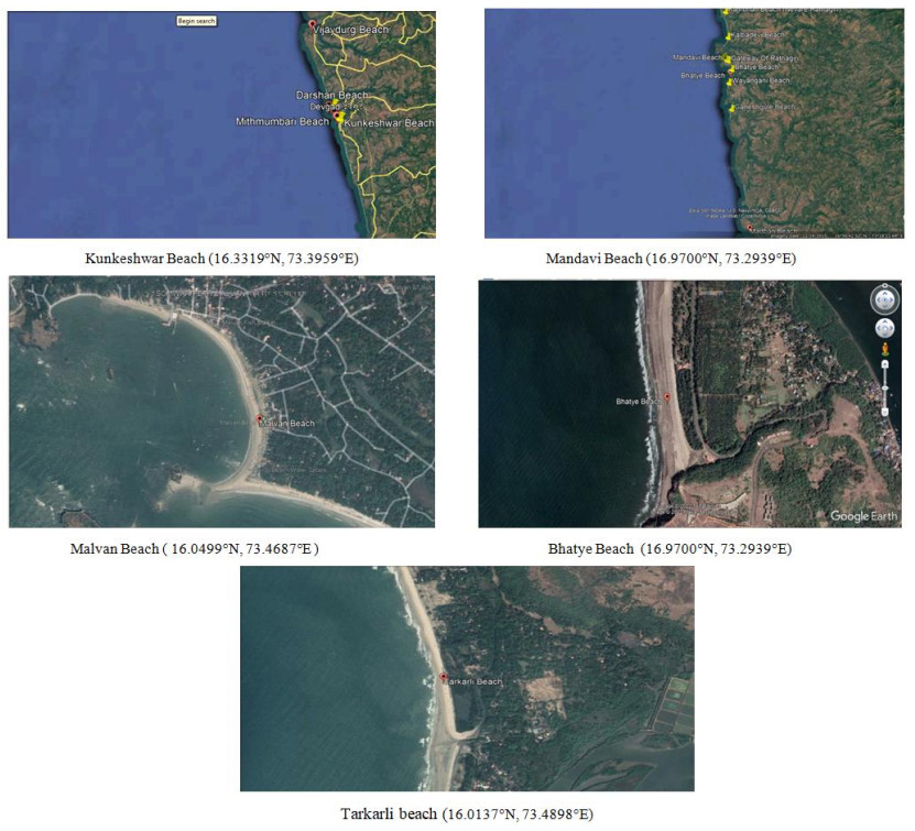
The recent marine algae study was carried out in the coastal region of Maharashtra, which is a district of Ratnagiri, Sindhudurg between 2021 and 2022. Water and algae samples were collected between September to October, mainly because to availability of algae is maximum in this period. The sampling locations were decided based on both previous work performed by researchers and on a literature review. The sampling sites were fixed based on the size of study area, sampling site accessibility, availability of algae on surface and substratum of the rock or wall. The microalgae were collected and preserved in plastic jar containing 3% to 4% formalin. The water samples were collected and specific physical and chemical parameters such as pH with pH meter, dissolved oxygen (mg/L) by DO meter, and temperature (Celsius) by digital thermometer were analyzed in situ. The remaining physical and chemical parameters were analyzed in the departmental research laboratory using standard methods outlined by the American Public Health Association (APHA). The collected micro algae were identified by a standard microscopy method using key references and with the help of algae experts. The main objective of the present research was to conduct extensive research on the collection and identification of diverse algal species in a coastal region to determine algal diversity, to determine the water quality standard and to measure the occurrence of algae in water.
Citation: Smita M. Pore, Vinayak P. Dhulap. Identification of marine micro algae in correlation with water quality assessment of coastal region of Maharashtra, India[J]. Clean Technologies and Recycling, 2023, 3(4): 257-266. doi: 10.3934/ctr.2023016
The recent marine algae study was carried out in the coastal region of Maharashtra, which is a district of Ratnagiri, Sindhudurg between 2021 and 2022. Water and algae samples were collected between September to October, mainly because to availability of algae is maximum in this period. The sampling locations were decided based on both previous work performed by researchers and on a literature review. The sampling sites were fixed based on the size of study area, sampling site accessibility, availability of algae on surface and substratum of the rock or wall. The microalgae were collected and preserved in plastic jar containing 3% to 4% formalin. The water samples were collected and specific physical and chemical parameters such as pH with pH meter, dissolved oxygen (mg/L) by DO meter, and temperature (Celsius) by digital thermometer were analyzed in situ. The remaining physical and chemical parameters were analyzed in the departmental research laboratory using standard methods outlined by the American Public Health Association (APHA). The collected micro algae were identified by a standard microscopy method using key references and with the help of algae experts. The main objective of the present research was to conduct extensive research on the collection and identification of diverse algal species in a coastal region to determine algal diversity, to determine the water quality standard and to measure the occurrence of algae in water.

| [1] | Appavu A, Thangavelu S, Muthukannan S, et al. (2016) Study of water quality parameters of cauvery river water in Erode region. J Global Biosci 5: 4556–4567. |
| [2] |
Sen B, Alp MT, Sonmez F, et al. (2013) Relationship of algae to water pollution and waste water treatment. Water Treat 14: 335–354. https://doi.org/10.5772/51927 doi: 10.5772/51927

|
| [3] | EPA, Drinking Water Health Advisory for Manganese. U.S. Environmental Protection Agency, 2004. Available from: https://www.epa.gov/sites/default/files/2014-09/documents/support_cc1_magnese_dwreport_0.pdf. |
| [4] | EPA, Secondary Drinking Water Regulations. U.S. Environmental Protection Agency, 2023. Available from: https://www.epa.gov/sdwa/secondary-drinking-water-standards-guidance-nuisance-chemicals. |
| [5] |
Ebrahimzadeh G, Alimohammadi M, Kahkah MRR, et al. (2021) Relationship between algae diversity and water quality-a case study: Chah Niemeh reservoir Southeast of Iran. J Environ Health Sci Eng 19: 437–443. https://doi.org/10.1007/s40201-021-00616-x doi: 10.1007/s40201-021-00616-x
|
| [6] | Abed IJ, Al-Hussieny AA, Kamel RF, et al. (2014) Environmental and identification study of algae present in three drinking water plants located on tigris river in Baghdad. Int J Adv Res 2: 895–900. |
| [7] |
Rahmanian N, Ali SHB, Homayoonfard M, et al. (2015) Analysis of physiochemical parameters to evaluate the drinking water quality in the State of Perak, Malaysia. J Chem 2015: 1–10. https://doi.org/10.1155/2015/716125 doi: 10.1155/2015/716125
|
| [8] |
Sarwa P, Verma SK (2017) Identification and characterization of green microalgae, Scenedesmus sp. MCC26 and Acutodesmus obliquus MCC33 isolated from industrial polluted site using morphological and molecular markers. Int J Appl Sci Biotechnol 5: 415–422. https://doi.org/10.3126/ijasbt.v5i4.18083 doi: 10.3126/ijasbt.v5i4.18083
|
| [9] |
Tian Y, Huang M (2019) An integrated web-based system for the monitoring and forecasting of coastal harmful algae blooms: Application to Shenzhen city, China. J Mar Sci Eng 7: 314. https://doi.org/10.3390/jmse7090314 doi: 10.3390/jmse7090314
|
| [10] | Narayanan RM, Sharmila KJ, Dharanirajan K (2016) Evaluation of marine water quality–a case study between cuddalore and pondicherry coast, India. Indian J Mar Sci 45: 517–532. |
| [11] |
Khalil S, Mahnashi MH, Hussain M, et al. (2021) Exploration and determination of algal role as Bioindicator to evaluate water quality–Probing fresh water algae. Saudi J Biol Sci 28: 5728–5737. https://doi.org/10.1016/j.sjbs.2021.06.004 doi: 10.1016/j.sjbs.2021.06.004
|
| [12] |
Rodrigues S, Pinto I, Formigo N, et al. (2021) Microalgae growth inhibition-based reservoirs water quality assessment to identify ecotoxicological risks. Water 13: 2605. https://doi.org/10.3390/w13192605 doi: 10.3390/w13192605
|


Figures(3) / Tables(2)
Smita M. Pore, Vinayak P. Dhulap. Identification of marine micro algae in correlation with water quality assessment of coastal region of Maharashtra, India[J]. Clean Technologies and Recycling, 2023, 3(4): 257-266. doi: 10.3934/ctr.2023016


 DownLoad: