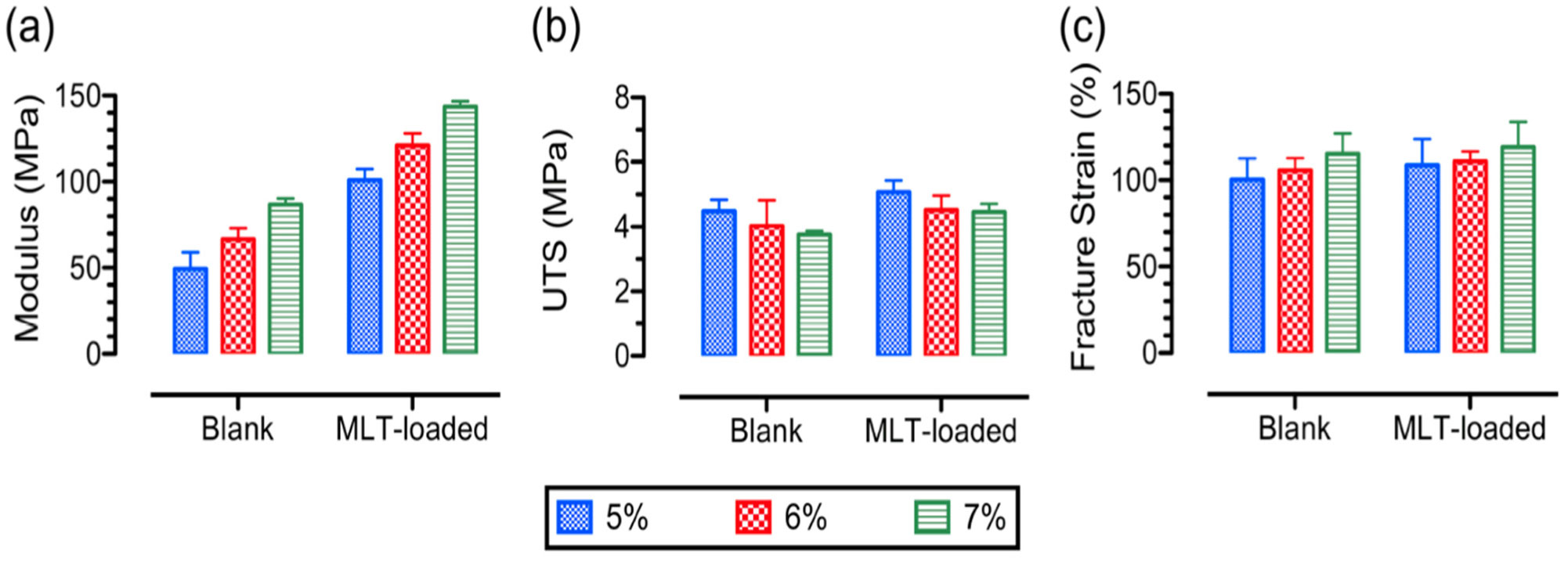
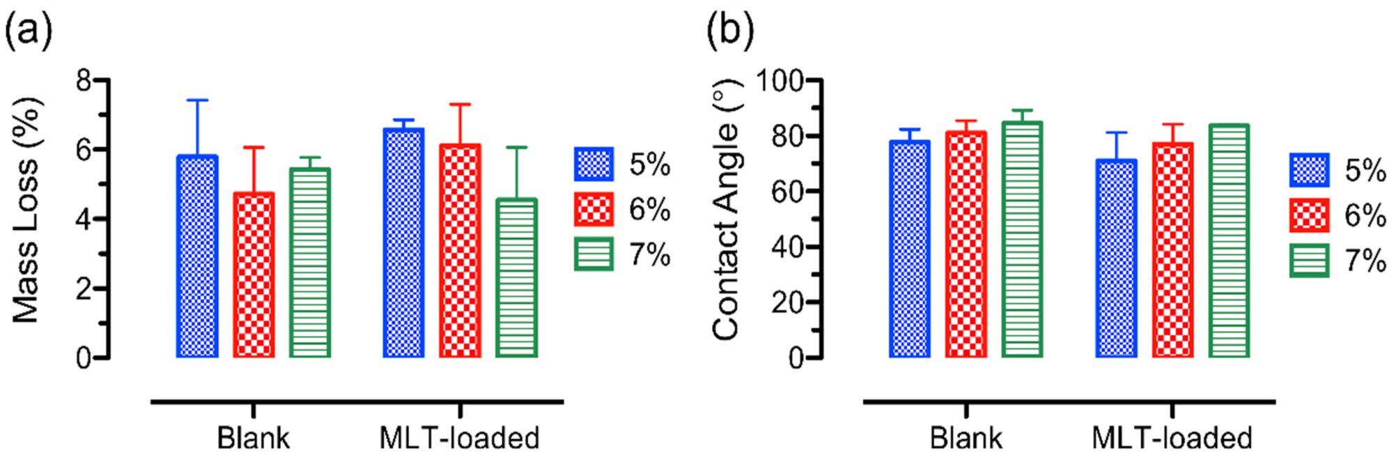
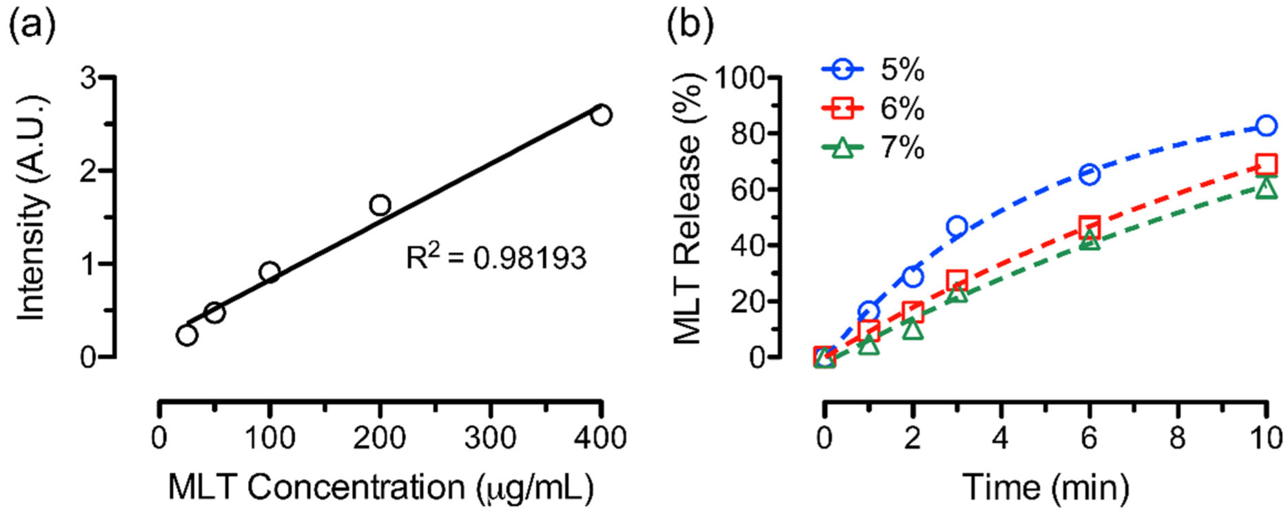
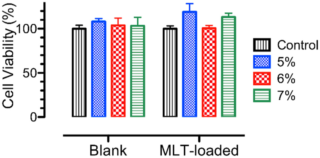
Water-soluble polymers possess great advantages in current drug delivery systems, such as fast delivery through polymer matrix dissolution as well as promoting solid dispersion of poorly water-soluble drugs. In this work, water-soluble polyvinyl alcohol (PVA) and polyethylene oxide (PEO) were blended (50/50) to electrospin with and without the incorporation of a model drug, melatonin (MLT), at various blend polymer concentrations. Results suggested that increasing blend PVA/PEO solution concentrations, up to 7 wt%, promoted the formation of smooth and defect-free drug-incorporating fibers with an average fiber diameter ranged from 300 to 700 nm. Mechanical properties of the blank and MLT-loaded PVA/PEO fibers showed dependence on fiber morphologies and fiber mat structures, due to polymer concentrations for electrospinning. Furthermore, the surface wettability of the blend PVA/PEO fibers were investigated and further correlated with the MLT release profile of the fibers. Results suggested that fiber mats with a more well-defined fiber structure promoted a linear release behavior within 10 minutes in vitro. These drug-incorporated fibers were compatible to human umbilical vein endothelial cells (HUVECs) up to 24 hours. In general, this work demonstrated the structure-property correlations of electrospun PVA/PEO fibers and their potential biomedical applications in fast delivery of small molecule drugs.
Citation: Rachel Emerine, Shih-Feng Chou. Fast delivery of melatonin from electrospun blend polyvinyl alcohol and polyethylene oxide (PVA/PEO) fibers[J]. AIMS Bioengineering, 2022, 9(2): 178-196. doi: 10.3934/bioeng.2022013
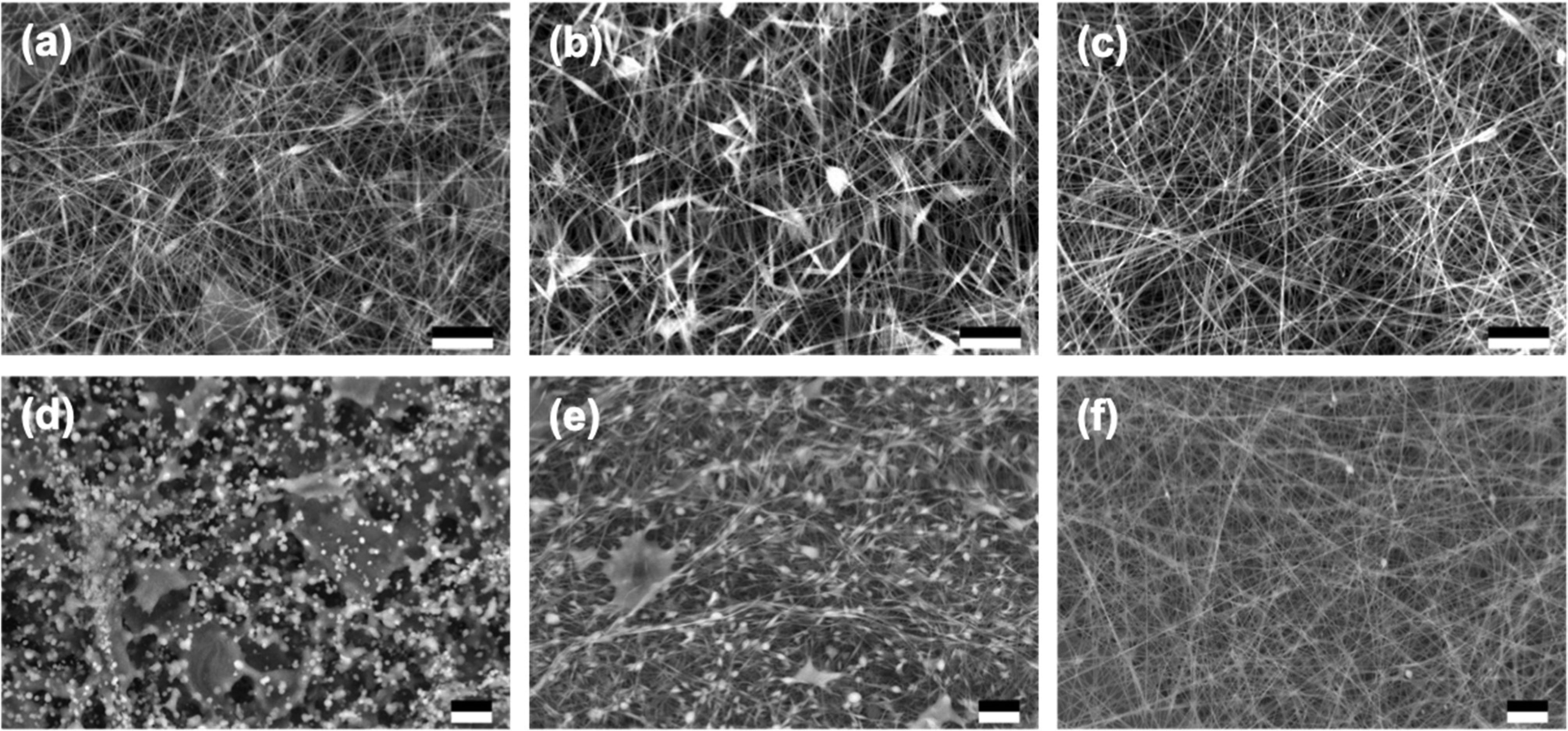
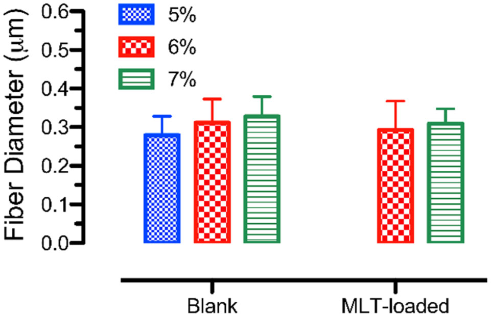
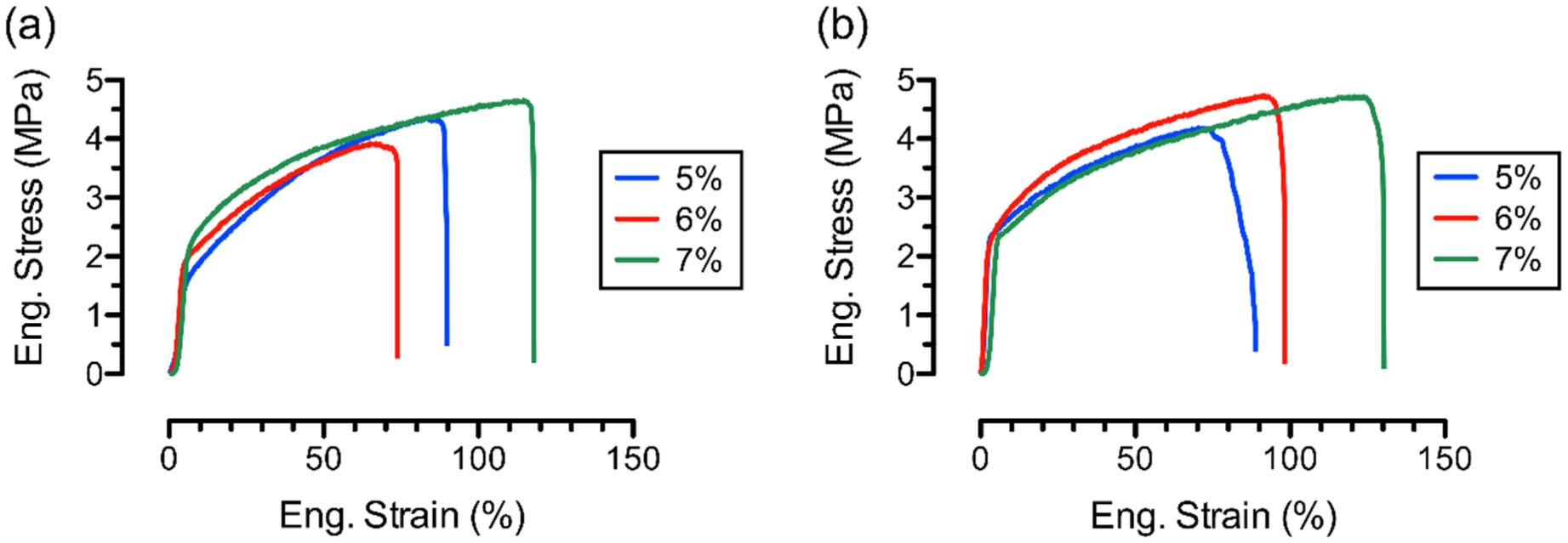
Water-soluble polymers possess great advantages in current drug delivery systems, such as fast delivery through polymer matrix dissolution as well as promoting solid dispersion of poorly water-soluble drugs. In this work, water-soluble polyvinyl alcohol (PVA) and polyethylene oxide (PEO) were blended (50/50) to electrospin with and without the incorporation of a model drug, melatonin (MLT), at various blend polymer concentrations. Results suggested that increasing blend PVA/PEO solution concentrations, up to 7 wt%, promoted the formation of smooth and defect-free drug-incorporating fibers with an average fiber diameter ranged from 300 to 700 nm. Mechanical properties of the blank and MLT-loaded PVA/PEO fibers showed dependence on fiber morphologies and fiber mat structures, due to polymer concentrations for electrospinning. Furthermore, the surface wettability of the blend PVA/PEO fibers were investigated and further correlated with the MLT release profile of the fibers. Results suggested that fiber mats with a more well-defined fiber structure promoted a linear release behavior within 10 minutes in vitro. These drug-incorporated fibers were compatible to human umbilical vein endothelial cells (HUVECs) up to 24 hours. In general, this work demonstrated the structure-property correlations of electrospun PVA/PEO fibers and their potential biomedical applications in fast delivery of small molecule drugs.

| [1] |
Szunerits S, Boukherroub R (2018) Heat: A highly efficient skin enhancer for transdermal drug delivery. Front Bioeng Biotechnol 6: 15. https://doi.org/10.3389/fbioe.2018.00015 
|
| [2] |
Alshehri S, Imam SS, Hussain A, et al. (2020) Potential of solid dispersions to enhance solubility, bioavailability, and therapeutic efficacy of poorly water-soluble drugs: newer formulation techniques, current marketed scenario and patents. Drug Deliv 27: 1625-1643. https://doi.org/10.1080/10717544.2020.1846638
|
| [3] |
Prajapati SK, Jain A, Jain A, et al. (2019) Biodegradable polymers and constructs: A novel approach in drug delivery. Eur Polym J 120: 109191. https://doi.org/10.1016/j.eurpolymj.2019.08.018
|
| [4] |
Waly AL, Abdelghany AM, Tarabiah AE (2021) Study the structure of selenium modified polyethylene oxide/polyvinyl alcohol (PEO/PVA) polymer blend. J Mater Res Technol 14: 2962-2969. https://doi.org/10.1016/j.jmrt.2021.08.078
|
| [5] |
Bala R, Khanna S, Pawar P (2014) Design optimization and in vitro - in vivo evaluation of orally dissolving strips of clobazam. J Drug Deliv 2014: 1-15. https://doi.org/10.1155/2014/392783
|
| [6] |
Yun YH, Lee BK, Park K (2015) Controlled drug delivery: Historical perspective for the next generation. J Controlled Release 219: 2-7. https://doi.org/10.1016/j.jconrel.2015.10.005
|
| [7] |
Chou S-F, Carson D, Woodrow KA (2015) Current strategies for sustaining drug release from electrospun nanofibers. J Controlled Release 220: 584-591. https://doi.org/10.1016/j.jconrel.2015.09.008
|
| [8] |
Gizaw M, Thompson J, Faglie A, et al. (2018) Electrospun fibers as a dressing material for drug and biological agent delivery in wound healing applications. Bioengineering 5: 9. https://doi.org/10.3390/bioengineering5010009
|
| [9] |
Chou S-F, Woodrow KA (2017) Relationships between mechanical properties and drug release from electrospun fibers of PCL and PLGA blends. J Mech Behav Biomed Mater 65: 724-733. https://doi.org/10.1016/j.jmbbm.2016.09.004
|
| [10] |
Ball C, Chou S-F, Jiang Y, et al. (2016) Coaxially electrospun fiber-based microbicides facilitate broadly tunable release of maraviroc. Mater Sci Eng C 63: 117-124. https://doi.org/10.1016/j.msec.2016.02.018
|
| [11] |
Bagheri M, Validi M, Gholipour A, et al. (2022) Chitosan nanofiber biocomposites for potential wound healing applications: Antioxidant activity with synergic antibacterial effect. Bioeng Transl Med 7: e10254. https://doi.org/10.1002/btm2.10254
|
| [12] |
Moroni I, Garcia-Bennett AE (2021) Effects of absorption kinetics on the catabolism of melatonin released from CAP-coated mesoporous silica drug delivery vehicles. Pharmaceutics 13: 1436. https://doi.org/10.3390/pharmaceutics13091436
|
| [13] |
Al-Zaqri N, Pooventhiran T, Alsalme A, et al. (2020) Structural and physico-chemical evaluation of melatonin and its solution-state excited properties, with emphasis on its binding with novel coronavirus proteins. J Mol Liq 318: 114082. https://doi.org/10.1016/j.molliq.2020.114082
|
| [14] |
Hawkins BC, Burnett E, Chou S-F (2022) Physicomechanical properties and in vitro release behaviors of electrospun ibuprofen-loaded blend PEO/EC fibers. Mater Today Commun 30: 103205. https://doi.org/10.1016/j.mtcomm.2022.103205
|
| [15] | ASTM D1708-18Standard test method for tensile properties of plastics by use of microtensile specimens, West Conshohocken, PA, ASTM International (2018). |
| [16] | ASTM D5034-21Standard test method for breaking strength and elongation of textile fabrics (grab test), West Conshohocken, PA, ASTM International (2021). |
| [17] |
Hekmati AH, Khenoussi N, Nouali H, et al. (2014) Effect of nanofiber diameter on water absorption properties and pore size of polyamide-6 electrospun nanoweb. Text Res J 84: 2045-2055. https://doi.org/10.1177/0040517514532160
|
| [18] |
Daescu M, Toulbe N, Baibarac M, et al. (2020) Photoluminescence as a complementary tool for UV-VIS spectroscopy to highlight the photodegradation of drugs: A case study on melatonin. Molecules 25: 3820. https://doi.org/10.3390/molecules25173820
|
| [19] |
Haro Durand L, Vargas G, Vera-Mesones R, et al. (2017) In vitro human umbilical vein endothelial cells response to ionic dissolution products from lithium-containing 45S5 bioactive glass. Materials 10: 740. https://doi.org/10.3390/ma10070740
|
| [20] |
Amariei N, Manea LR, Bertea AP, et al. (2017) The influence of polymer solution on the properties of electrospun 3D nanostructures. IOP Conf Ser Mater Sci Eng 209: 012092. https://doi.org/10.1088/1757-899X/209/1/012092
|
| [21] |
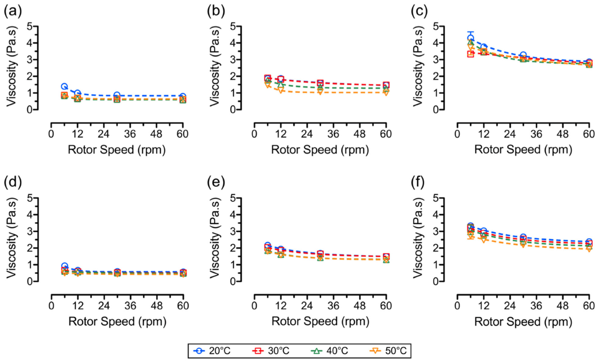
Datta R, Yelash L, Schmid F, et al. (2021) Shear-thinning in oligomer melts—Molecular origins and applications. Polymers 13: 2806. https://doi.org/10.3390/polym13162806
|
| [22] |
Mirtič J, Balažic H, Zupančič Š, et al. (2019) Effect of solution composition variables on electrospun alginate nanofibers: Response surface analysis. Polymers 11: 692. https://doi.org/10.3390/polym11040692
|
| [23] |
Briscoe B, Luckham P, Zhu S (2000) The effects of hydrogen bonding upon the viscosity of aqueous poly(vinyl alcohol) solutions. Polymer 41: 3851-3860. https://doi.org/10.1016/S0032-3861(99)00550-9
|
| [24] |
Vlachou M, Siamidi A, Anagnostopoulou D, et al. (2022) Modified release of the pineal hormone melatonin from matrix tablets containing poly(L-lactic acid) and its PLA-co-PEAd and PLA-co-PBAd copolymers. Polymers 14: 1504. https://doi.org/10.3390/polym14081504
|
| [25] |
Angel N, Li S, Yan F, et al. (2022) Recent advances in electrospinning of nanofibers from bio-based carbohydrate polymers and their applications. Trends Food Sci Technol 120: 308-324. https://doi.org/10.1016/j.tifs.2022.01.003
|
| [26] |
Son WK, Youk JH, Lee TS, et al. (2004) The effects of solution properties and polyelectrolyte on electrospinning of ultrafine poly(ethylene oxide) fibers. Polymer 45: 2959-2966. https://doi.org/10.1016/j.polymer.2004.03.006
|
| [27] |
Filip P, Peer P (2019) Characterization of poly(ethylene oxide) nanofibers—Mutual relations between mean diameter of electrospun nanofibers and solution characteristics. Processes 7: 948. https://doi.org/10.3390/pr7120948
|
| [28] |
Ziyadi H, Baghali M, Bagherianfar M, et al. (2021) An investigation of factors affecting the electrospinning of poly (vinyl alcohol)/kefiran composite nanofibers. Adv Compos Hybrid Mater 4: 768-779. https://doi.org/10.1007/s42114-021-00230-3
|
| [29] |
Mwiiri FK, Daniels R (2020) Influence of PVA molecular weight and concentration on electrospinnability of birch bark extract-loaded nanofibrous scaffolds intended for enhanced wound healing. Molecules 25: 4799. https://doi.org/10.3390/molecules25204799
|
| [30] |
Cho D, Netravali AN, Joo YL (2012) Mechanical properties and biodegradability of electrospun soy protein isolate/PVA hybrid nanofibers. Polym Degrad Stab 97: 747-754. https://doi.org/10.1016/j.polymdegradstab.2012.02.007
|
| [31] |
Amjadi M, Fatemi A (2020) Tensile behavior of high-density polyethylene including the effects of processing technique, thickness, temperature, and strain rate. Polymers 12: 1857. https://doi.org/10.3390/polym12091857
|
| [32] | Séguéla R (2007) Plasticity of semi-crystalline polymers: crystal slip versus melting-recrystallization. E-Polym 7: 32. https://doi.org/10.1515/epoly.2007.7.1.382 |
| [33] |
Devangamath SS, Lobo B, Masti SP, et al. (2020) Thermal, mechanical, and AC electrical studies of PVA–PEG–Ag2S polymer hybrid material. J Mater Sci Mater Electron 31: 2904-2917. https://doi.org/10.1007/s10854-019-02835-3
|
| [34] |
Rashid TU, Gorga RE, Krause WE (2021) Mechanical properties of electrospun fibers—A critical review. Adv Eng Mater 23: 2100153. https://doi.org/10.1002/adem.202100153
|
| [35] |
Morel A, Domaschke S, Urundolil Kumaran V, et al. (2018) Correlating diameter, mechanical and structural properties of poly(
|
| [36] | Parab RS, Rao GK (2019) Understanding the mechanical properties of polymer blends in the presence of plasticizers and other additives. Int J Pharm Sci Rev Res 54: 84-91. |
| [37] |
Croisier F, Duwez A-S, Jérôme C, et al. (2012) Mechanical testing of electrospun PCL fibers. Acta Biomater 8: 218-224. https://doi.org/10.1016/j.actbio.2011.08.015
|
| [38] |
Ghasemi M, Singapati AY, Tsianou M, et al. (2017) Dissolution of semicrystalline polymer fibers: Numerical modeling and parametric analysis. AIChE J 63: 1368-1383. https://doi.org/10.1002/aic.15615
|
| [39] |
Hirsch E, Pantea E, Vass P, et al. (2021) Probiotic bacteria stabilized in orally dissolving nanofibers prepared by high-speed electrospinning. Food Bioprod Process 128: 84-94. https://doi.org/10.1016/j.fbp.2021.04.016
|
| [40] |
Zhang J, Yan X, Tian Y, et al. (2020) Synthesis of a new water-soluble melatonin derivative with low toxicity and a strong effect on sleep aid. ACS Omega 5: 6494-6499. https://doi.org/10.1021/acsomega.9b04120
|
| [41] |
Khan MQ, Kharaghani D, Nishat N, et al. (2019) Preparation and characterizations of multifunctional PVA/ZnO nanofibers composite membranes for surgical gown application. J Mater Res Technol 8: 1328-1334. https://doi.org/10.1016/j.jmrt.2018.08.013
|
| [42] |
Song X, Gao Z, Ling F, et al. (2012) Controlled release of drug via tuning electrospun polymer carrier. J Polym Sci Part B Polym Phys 50: 221-227. https://doi.org/10.1002/polb.23005
|
| [43] |
Mihailiasa M, Caldera F, Li J, et al. (2016) Preparation of functionalized cotton fabrics by means of melatonin loaded β-cyclodextrin nanosponges. Carbohydr Polym 142: 24-30. https://doi.org/10.1016/j.carbpol.2016.01.024
|
| [44] |
Gulino EF, Citarrella MC, Maio A, et al. (2022) An innovative route to prepare in situ graded crosslinked PVA graphene electrospun mats for drug release. Compos Part Appl Sci Manuf 155: 106827. https://doi.org/10.1016/j.compositesa.2022.106827
|
| [45] |
Torres-Martínez EJ, Vera-Graziano R, Cervantes-Uc JM, et al. (2020) Preparation and characterization of electrospun fibrous scaffolds of either PVA or PVP for fast release of sildenafil citrate. E-Polym 20: 746-758. https://doi.org/10.1515/epoly-2020-0070
|
| [46] |
Carvalho LD de, Peres BU, Maezono H, et al. (2019) Doxycycline release and antibacterial activity from PMMA/PEO electrospun fiber mats. J Appl Oral Sci 27: e20180663. https://doi.org/10.1590/1678-7757-2018-0663
|
| [47] |
Eskitoros-Togay ŞM, Bulbul YE, Tort S, et al. (2019) Fabrication of doxycycline-loaded electrospun PCL/PEO membranes for a potential drug delivery system. Int J Pharm 565: 83-94. https://doi.org/10.1016/j.ijpharm.2019.04.073
|
| [48] |
Yu D-G, Shen X-X, Branford-White C, et al. (2009) Oral fast-dissolving drug delivery membranes prepared from electrospun polyvinylpyrrolidone ultrafine fibers. Nanotechnology 20: 055104. https://doi.org/10.1088/0957-4484/20/5/055104
|
| [49] |
Samprasit W, Akkaramongkolporn P, Ngawhirunpat T, et al. (2015) Fast releasing oral electrospun PVP/CD nanofiber mats of taste-masked meloxicam. Int J Pharm 487: 213-222. https://doi.org/10.1016/j.ijpharm.2015.04.044
|
| [50] |
Huang C-Y, Hu K-H, Wei Z-H (2016) Comparison of cell behavior on pva/pva-gelatin electrospun nanofibers with random and aligned configuration. Sci Rep 6: 37960. https://doi.org/10.1038/srep37960
|
| [51] |
Yang JM, Yang JH, Tsou SC, et al. (2016) Cell proliferation on PVA/sodium alginate and PVA/poly(γ-glutamic acid) electrospun fiber. Mater Sci Eng C 66: 170-177. https://doi.org/10.1016/j.msec.2016.04.068
|
| [52] |
Carrasco-Torres G, Valdés-Madrigal M, Vásquez-Garzón V, et al. (2019) Effect of silk fibroin on cell viability in electrospun scaffolds of polyethylene oxide. Polymers 11: 451. https://doi.org/10.3390/polym11030451
|
| [53] |
Cerqueira A, Romero-Gavilán F, Araújo-Gomes N, et al. (2020) A possible use of melatonin in the dental field: Protein adsorption and in vitro cell response on coated titanium. Mater Sci Eng C 116: 111262. https://doi.org/10.1016/j.msec.2020.111262
|
| [54] | Cheng J, Yang H, Gu C, et al. (2018) Melatonin restricts the viability and angiogenesis of vascular endothelial cells by suppressing HIF-1α/ROS/VEGF. Int J Mol Med 43: 945-955. https://doi.org/10.3892/ijmm.2018.4021 |
Figures(8) / Tables(1)

Rachel Emerine, Shih-Feng Chou. Fast delivery of melatonin from electrospun blend polyvinyl alcohol and polyethylene oxide (PVA/PEO) fibers[J]. AIMS Bioengineering, 2022, 9(2): 178-196. doi: 10.3934/bioeng.2022013


 DownLoad: