Anomaly detection strategies in industrial control systems mainly investigate the transmitting network traffic called network intrusion detection system. However, The measurement intrusion detection system inspects the sensors data integrated into the supervisory control and data acquisition center to find any abnormal behavior. An approach to detect anomalies in the measurement data is training supervised learning models that can learn to classify normal and abnormal data. But, a labeled dataset consisting of abnormal behavior, such as attacks, or malfunctions is extremely hard to achieve. Therefore, the unsupervised learning strategy that does not require labeled data for being trained can be helpful to tackle this problem. This study evaluates the performance of unsupervised learning strategies in anomaly detection using measurement data in control systems. The most accurate algorithms are selected to train unsupervised learning models, and the results show an accuracy of 98% in stealthy attack detection.
Citation: Sohrab Mokhtari, Kang K Yen. Measurement data intrusion detection in industrial control systems based on unsupervised learning[J]. Applied Computing and Intelligence, 2021, 1(1): 61-74. doi: 10.3934/aci.2021004
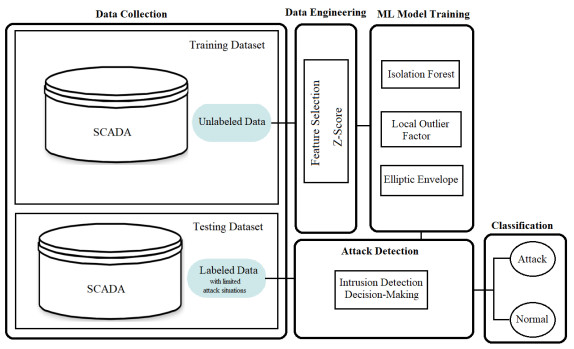
Anomaly detection strategies in industrial control systems mainly investigate the transmitting network traffic called network intrusion detection system. However, The measurement intrusion detection system inspects the sensors data integrated into the supervisory control and data acquisition center to find any abnormal behavior. An approach to detect anomalies in the measurement data is training supervised learning models that can learn to classify normal and abnormal data. But, a labeled dataset consisting of abnormal behavior, such as attacks, or malfunctions is extremely hard to achieve. Therefore, the unsupervised learning strategy that does not require labeled data for being trained can be helpful to tackle this problem. This study evaluates the performance of unsupervised learning strategies in anomaly detection using measurement data in control systems. The most accurate algorithms are selected to train unsupervised learning models, and the results show an accuracy of 98% in stealthy attack detection.

| [1] |
A. Abbaspour, S. Mokhtari, A. Sargolzaei, K. K. Yen, A survey on active fault-tolerant control systems, Electronics, 9 (2021), 1513. doi: 10.3390/electronics9091513 doi: 10.3390/electronics9091513

|
| [2] |
N. Sultana, N. Chilamkurti, W. Peng, R. Alhadad, Survey on SDN based network intrusion detection system using machine learning approaches, Peer-to-Peer Netw. Appl., 12 (2019), 493–501. doi: 10.1007/s12083-017-0630-0 doi: 10.1007/s12083-017-0630-0
|
| [3] |
S. Mokhtari, A. Abbaspour, K. K. Yen, A. Sargolzaei, A machine learning approach for anomaly detection in industrial control systems based on measurement data, Electronics, 10 (2021), 407. doi: 10.3390/electronics10040407 doi: 10.3390/electronics10040407
|
| [4] |
V. Chandola, A. Banerjee, V. Kumar, Anomaly detection: A survey, ACM comput. surv. (CSUR), 41 (2009), 1–58. doi: 10.1145/1541880.1541882 doi: 10.1145/1541880.1541882
|
| [5] |
K. Paridari, N. O'Mahony, A. Mady, R. Chabukswar, M. Boubekeur, H. Sandberg, A framework for attack-resilient industrial control systems: Attack detection and controller reconfiguration, P. IEEE, 106 (2017), 113–128. doi: 10.1109/JPROC.2017.2725482 doi: 10.1109/JPROC.2017.2725482
|
| [6] |
J. Goh, S. Adepu, M. Tan, Z. S. Lee, Anomaly detection in cyber physical systems using recurrent neural networks, 2017 IEEE 18th International Symposium on High Assurance Systems Engineering (HASE), (2017), 140–145. doi: 10.1109/HASE.2017.36 doi: 10.1109/HASE.2017.36
|
| [7] |
A. Javaid, Q. Niyaz, W. Sun, M. Alam, A deep learning approach for network intrusion detection system, Eai Endorsed Transactions on Security and Safety, 3 (2016). doi: 10.4108/eai.3-12-2015.2262516 doi: 10.4108/eai.3-12-2015.2262516
|
| [8] |
H. Choi, M. Kim, G. Lee, W. Kim, Unsupervised learning approach for network intrusion detection system using autoencoders, The Journal of Supercomputing, 75 (2019), 5597–5621. doi: 10.1007/s11227-019-02805-w doi: 10.1007/s11227-019-02805-w
|
| [9] | M. Masson, Darktrace OT threat finds: Detecting an advanced ICS attack targeting an international airport, Aug., 2007. Available from: http://shorturl.at/nuJ19. |
| [10] |
Y. Liu, Y. Mu, K. Chen, Y. Li, J. Guo, Daily activity feature selection in smart homes based on pearson correlation coefficient, Neural Process. Lett., (2020), 1–17. doi: 10.1007/s11063-019-10185-8 doi: 10.1007/s11063-019-10185-8
|
| [11] |
S. Bornelöv, J. Komorowski, Selection of significant features using Monte Carlo feature selection, Challenges in Computational Statistics and Data Mining, (2016), 25–38. doi: 10.1007/978-3-319-18781-5_2 doi: 10.1007/978-3-319-18781-5_2
|
| [12] |
Q. Guo, W. Wu, D. L. Massart, C. Boucon, S. De Jong, Feature selection in principal component analysis of analytical data, Chemometr. Intell. Lab., 61 (2002), 123–132. doi: 10.1016/S0169-7439(01)00203-9 doi: 10.1016/S0169-7439(01)00203-9
|
| [13] |
J. G. Dy, C. E. Brodley, Feature selection for unsupervised learning, J. Mach. Learn. Res., 5 (2004), 845–889. doi: 10.5555/1005332.1016787 doi: 10.5555/1005332.1016787
|
| [14] |
Y. Li, B. Lu, Z. Wu, Hierarchical fuzzy filter method for unsupervised feature selection, J. Intell. Fuzzy Syst., 18 (2007), 157–169. doi: 10.5555/1368376.1368381 doi: 10.5555/1368376.1368381
|
| [15] | Z table website provides all required information for using Z-test. Aug., 2021. Available from: https://www.ztable.net. |
| [16] |
F. T. Liu, K. M. Ting, Z. Zhou, Isolation forest, 2008 eighth ieee international conference on data mining, (2008), 413–422. doi: 10.1109/ICDM.2008.17 doi: 10.1109/ICDM.2008.17
|
| [17] |
M. Wu, C. Jermaine, Outlier detection by sampling with accuracy guarantees, Proceedings of the 12th ACM SIGKDD international conference on Knowledge discovery and data mining, (2006), 767–772. doi: 10.1145/1150402.1150501 doi: 10.1021/ie302042c
|
| [18] |
H. Ma, Y. Hu, H. Shi, Fault detection and identification based on the neighborhood standardized local outlier factor method, Ind. Eng. Chem. Res., 52 (2013), 2389–2402. doi: 10.1021/ie302042c doi: 10.1021/ie302042c
|
| [19] |
V. Kotu, B. Deshpande, Chapter 13 - Anomaly Detection, Data Science (Second Edition), (2019), 447–465. doi: 10.1016/B978-0-12-814761-0.00013-7 doi: 10.1016/B978-0-12-814761-0.00013-7
|
| [20] |
M. Ashrafuzzaman, S. Das, A. A. Jillepalli, Y. Chakhchoukh, F. T. Sheldon, Elliptic Envelope Based Detection of Stealthy False Data Injection Attacks in Smart Grid Control Systems, 2020 IEEE Symposium Series on Computational Intelligence (SSCI), (2020), 1131–1137. doi: 10.1109/SSCI47803.2020.9308523 doi: 10.1109/SSCI47803.2020.9308523
|
| [21] |
P. J. Rousseeuw, K. V. Driessen, A fast algorithm for the minimum covariance determinant estimator, Technometrics, 41 (1999), 212–223. doi: 10.1080/00401706.1999.10485670 doi: 10.1080/00401706.1999.10485670
|
| [22] |
P. C. Mahalanobis, On the generalized distance in statistics, National Institute of Science of India, 1936. doi: 10.1007/s13171-019-00164-5 doi: 10.1007/s13171-019-00164-5
|
| [23] |
M. Sokolova, G. Lapalme, A systematic analysis of performance measures for classification tasks, Inform. process. manag., 45 (2009), 427–437. doi: 10.1016/j.ipm.2009.03.002 doi: 10.1016/j.ipm.2009.03.002
|
| [24] |
N. V. Chawla, K. W. Bowyer, L. O. Hall, W. P. Kegelmeyer, SMOTE: synthetic minority over-sampling technique, J. artif. intell. res., 16 (2002), 321–357. doi: 10.5555/1622407.1622416 doi: 10.5555/1622407.1622416
|
| [25] |
H. Shin, W. Lee, J. Yun, H. Kim, HAI 1.0: HIL-based Augmented ICS Security Dataset, 13th $USENIX$ Workshop on Cyber Security Experimentation and Test ($CSET$ 20), 2020. doi: 10.5555/3485754.3485755 doi: 10.5555/3485754.3485755
|
| [26] | S. Choi, HIL-based Augmented ICS (HAI) Security Dataset, The Affiliated Institute of ETRI, South Korea, 2020. Available from: https://github.com/icsdataset/hai. |
| [27] |
H. Shin, W. Lee, J. Yun, H. Kim, Implementation of programmable CPS testbed for anomaly detection, 12th USENIX Workshop on Cyber Security Experimentation and Test (CSET 19), 2019. doi: 10.5555/3359012.3359014 doi: 10.5555/3359012.3359014
|
| [28] |
W. Hwang, J. Yun, J. Kim, H. Kim, Time-series aware precision and recall for anomaly detection: considering variety of detection result and addressing ambiguous labeling, Proceedings of the 28th ACM International Conference on Information and Knowledge Management, (2019), 2241–2244. doi: 10.1145/3357384.3358118 doi: 10.1145/3357384.3358118
|


Figures(4) / Tables(1)
Sohrab Mokhtari, Kang K Yen. Measurement data intrusion detection in industrial control systems based on unsupervised learning[J]. Applied Computing and Intelligence, 2021, 1(1): 61-74. doi: 10.3934/aci.2021004


 DownLoad: