Figure 1.
Issues with current landfills [1].


Citation: Jian Zou, Fulton T. Crews. Glutamate/NMDA excitotoxicity and HMGB1/TLR4 neuroimmune toxicity converge as components of neurodegeneration[J]. AIMS Molecular Science, 2015, 2(2): 77-100. doi: 10.3934/molsci.2015.2.77
| [1] | Sumera Naz, Muhammad Akram, Mohammed M. Ali Al-Shamiri, Mohammed M. Khalaf, Gohar Yousaf . A new MAGDM method with 2-tuple linguistic bipolar fuzzy Heronian mean operators. Mathematical Biosciences and Engineering, 2022, 19(4): 3843-3878. doi: 10.3934/mbe.2022177 |
| [2] | Muhammad Akram, Ayesha Khan, Uzma Ahmad, José Carlos R. Alcantud, Mohammed M. Ali Al-Shamiri . A new group decision-making framework based on 2-tuple linguistic complex $ q $-rung picture fuzzy sets. Mathematical Biosciences and Engineering, 2022, 19(11): 11281-11323. doi: 10.3934/mbe.2022526 |
| [3] | Ayesha Khan, Muhammad Akram, Uzma Ahmad, Mohammed M. Ali Al-Shamiri . A new multi-objective optimization ratio analysis plus full multiplication form method for the selection of an appropriate mining method based on 2-tuple spherical fuzzy linguistic sets. Mathematical Biosciences and Engineering, 2023, 20(1): 456-488. doi: 10.3934/mbe.2023021 |
| [4] | Muhammad Akram, G. Muhiuddin, Gustavo Santos-García . An enhanced VIKOR method for multi-criteria group decision-making with complex Fermatean fuzzy sets. Mathematical Biosciences and Engineering, 2022, 19(7): 7201-7231. doi: 10.3934/mbe.2022340 |
| [5] | Han Wu, Junwu Wang, Sen Liu, Tingyou Yang . Research on decision-making of emergency plan for waterlogging disaster in subway station project based on linguistic intuitionistic fuzzy set and TOPSIS. Mathematical Biosciences and Engineering, 2020, 17(5): 4825-4851. doi: 10.3934/mbe.2020263 |
| [6] | Ghous Ali, Adeel Farooq, Mohammed M. Ali Al-Shamiri . Novel multiple criteria decision-making analysis under $ m $-polar fuzzy aggregation operators with application. Mathematical Biosciences and Engineering, 2023, 20(2): 3566-3593. doi: 10.3934/mbe.2023166 |
| [7] | Bo Sun, Ming Wei, Wei Wu, Binbin Jing . A novel group decision making method for airport operational risk management. Mathematical Biosciences and Engineering, 2020, 17(3): 2402-2417. doi: 10.3934/mbe.2020130 |
| [8] | Xiangzheng Fu, Yifan Chen, Sha Tian . DlncRNALoc: A discrete wavelet transform-based model for predicting lncRNA subcellular localization. Mathematical Biosciences and Engineering, 2023, 20(12): 20648-20667. doi: 10.3934/mbe.2023913 |
| [9] | Miin-Shen Yang, Wajid Ali . Fuzzy Gaussian Lasso clustering with application to cancer data. Mathematical Biosciences and Engineering, 2020, 17(1): 250-265. doi: 10.3934/mbe.2020014 |
| [10] | Jianzhong Shi, Ying Song . Mathematical analysis of a simplified general type-2 fuzzy PID controller. Mathematical Biosciences and Engineering, 2020, 17(6): 7994-8036. doi: 10.3934/mbe.2020406 |
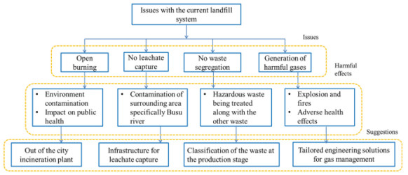
Manchester has a rich industrial heritage, a very diverse economy and a center for cultural industries, retail, transport, logistics, finance and manufacturing. Manufacturing companies rely on efficient and optimized production methods to create their products. But even the most efficient method of manufacturing plants inevitably generates some form of waste. The selection of the best place to dispose of the waste from manufacturing plants requires the need to first understand the type of waste. There are three main types of waste in manufacturing: solid waste, chemical waste and toxic waste. Solid waste includes paper, metal or carbon-based materials that are leftover after basic manufacturing processes have been completed. Some types of waste can be recycled and some cannot be recycled; the latter must be undergo proper disposal; otherwise, it will endanger the health of the workers. The second category is chemical waste, which includes the waste of residual chemicals. Some manufacturing processes may generate large amounts of chemical waste. Solid waste can be placed in the bin, but chemical waste should be handled in a specific way to prevent the dangerous effects of these chemicals. The third is toxic waste, which is a by-product of many manufacturing processes. We cannot reduce the toxicity of certain types of waste, but we should ensure that these toxic substances do not contaminate the surrounding environment. Some other types of waste are manufacturing waste, green waste, organic waste, metal and plastic waste, etc. Manufacturing waste includes dust, sand, broken glass, etc. Green garbage includes trees, leaves, grass, fruit, wood, etc. Organic waste includes food, leftover manure, straw, etc. Metal and plastic waste include bottle caps, batteries, etc. The form of waste that cannot be reused or recycled is often thrown into landfills. Landfills can be found all over the UK, in particular, Manchester has a lot of landfills. Some use the "landfill" method, and some use the "land-raising" method. Landfills are designed in such a way that the risk of contaminating the environment is minimized. They should be built away from industrial and residential areas. Although, landfills are a good source of waste disposal, but there are also some drawbacks. The main issues with landfills as follows:
1. toxins,
2. leachates,
3. greenhouse gases.
Electronic material when it becomes waste, contains toxic substances. These toxins leach into the soil and become hazardous. This leachate pollutes the groundwater and waterways. Landfills contain a lot of waste that can create leachates and become harmful to the environment. Some secondary side effects of landfills include the following:
1. nauseous odors,
2. unpleasant view,
3. rat and seagull infestations.
Even though it has a lot of disadvantages, it is still necessary because with increasing population waste is increasing day by day. Even with increasing recycling rates, it is still general waste which is to be disposed of in landfills. But there are a lot of problems with the current landfill system. Some of the issues with the current landfill system according to Doaemo et al. [1] are shown in Figure 1. Choosing the appropriate location for a landfill is very important because a wrong site selection causes a lot of health issues. The main objective of this research article is to propose the best method for the solid waste disposal location selection (SWDLS) problem of manufacturing plants in Manchester. The proposed methodology is based on the use of the weighted aggregated sum product assessment (WASPAS) method with 2-tuple linguistic Fermatean fuzzy sets (2TLFFSs). According to the ratings given by decision-makers (DMs), the simple multi-attribute rating technique (SMART) [2] is used to get the criteria weights. This method is also developed in many other fuzzy environments.
Zadeh [3] introduced the concept of fuzzy sets in 1965. The concept of an intuitionistic fuzzy set (IFS) was proposed by Atanassov [4] in 1986. Szmidt and Kacprzyk [5] introduced the medical applications of IFSs. Further, Yager [6] proposed the concept of a Pythagorean fuzzy set (PFS). PFS models are more powerful than IFS models in addressing real-world applications, but these collections have some limitations. Some applications may contain the decision maker's opinion as $ (0.8, 0.9) $. In such cases, PFSs and IFSs failed to apply. To overcome the limitations of IFSs and PFSs, Senapati and Yager [7] introduced Fermatean fuzzy sets (FFSs). The FFSs are those sets in which the cube sum of the membership degree (MD) and non-MD is less than or equal to 1. Senapati and Yager introduced the solution of some multi-criteria decision-making (MCDM) problems based on FFSs [8,9]. The utilization of FFSs in MAGDM (multi-attribute group decision-making) approaches have been proposed in [10,11]. Liu et al. [12] proposed an MAGDM method with probabilistic linguistic information based on an adaptive consensus reaching model and evidential reasoning. Liu et al. [13] presented an opinion dynamics and minimum adjustment-driven consensus model for multi-criteria large-scale group decision making under a novel social trust propagation mechanism. Liu et al. [14] proposed MCDM with incomplete weights based on 2-D uncertain linguistic Choquet integral operators.
The 2-tuple linguistic representation model was first proposed by Herrera and Martinez [15,16]. Several decision methods based on 2-tuple linguistic data have been presented. Fazi et al. [17] introduced worst-case methods and Hamacher aggregation operations for an intuitive 2-tuple linguistic set. Herrera and Herrera-Viedma [18] introduced the linguistic decision analysis procedure for solving decision problems with linguistic information. Recently, many applications for MAGDM issues have been developed [19,20] Zavadskas et al. [21] introduced the WASPAS method to solve the MAGDM problem. It is a combination of two models i.e., the weighted aggregated sum model (WeSM) and weighted aggregated product model (WePM). WASPAS is more precise than the WePM and WeSM. Zavadskas et al. [22] considered the single-valued neurotrophic WASPAS and discussed its applications in alternative site construction. Mishra et al. [23] presented a hesitant fuzzy HF WASPAS and illustrated its application in green supplier selection. Schitea et al. [24] discussed intuitionistic fuzzy (IF) WASPAS-COPRAS (COmplex PRoportional ASsessment)-EDAS (Evaluation based on Distance from Average Solution) and its application in site selection. Mardani et al. [25] described HF-strengths, Weaknesses, Opportunities, and Threats (SWOT)-stepwise weight assessment ratio analysis (SWARA)-WASPAS and its application in the assessment of digital technologies intervention. Akram and Niaz [26] recently proposed a 2-tuple linguistic Fermatean fuzzy (2TLFF) decision-making method based on combined compromise solution with criteria importance through inter-criteria correlation for drip irrigation system analysis. Rani et al. [27] studied the IF type-2 WASPAS and its application in physician selection. The existing studies based on the WASPAS method are shown in Table 1.
| Authors | Year | Significance influence |
| Zavadskas et al. [21] | 2012 | Proposed optimization of WASPAS |
| Antucheviciene et al. [28] | 2013 | Introduced MCDM methods WASPAS and MULTIMOORA |
| Lashgari et al. [29] | 2014 | Determined outsourcing strategies using QSPM and WASPAS methods |
| Zavadskas et al. [30] | 2014 | Designed WASPAS with interval-valued IF numbers |
| Chakraborty and Saparauskas [31] | 2014 | Proposed WASPAS method in manufacturing decision making |
| Chakraborty et al.[32] | 2015 | Studied WASPAS method as a MCDM tool |
| Zavadskas et al. [22] | 2015 | Presented the single-valued neurotrophic WASPAS |
| Zavadskas et al. [33] | 2015 | Studied WASPAS method as an optimization tool |
| Karabasevic et al. [34] | 2016 | Proposed a personnel selection method based on SWARA and WASPAS |
| Zavadskas et al. [35] | 2016 | Presented a multi-attribute assessment using WASPAS |
| Mardani et al. [36] | 2017 | Described a systematic review of SWARA and WASPAS |
| Mardani et al. [25] | 2017 | Introduced HF-SWOT-SWARA-WASPAS |
| Bausys and Juodagalvien [37] | 2017 | Investigated garage location selection using WASPAS-SVNS method |
| Stanujki and Karabasevi [38] | 2018 | Designed extension of the WASPAS method with IF numbers |
| Turskis et al. [39] | 2019 | Presented an F-WASPAS-based approach |
| Mishra et al. [23] | 2019 | Proposed the HF WASPAS |
| Schitea et al. [24] | 2019 | Described IF-WASPAS-COPRAS-EDAS |
| Gundogdu and Kahraman [40] | 2019 | Introduced WASPAS with spherical fuzzy sets |
| Dehshiri and Aghaei [41] | 2019 | Examined fuzzy Delphi, SWARA and WASPAS |
| Rani and Mishra [42] | 2020 | Proposed q-rung orthopair WASPAS |
| Mohagheghi and Mousavi [43] | 2020 | Introduced IVPF D-WASPAS |
| Rani et al. [27] | 2020 | Presented IF type-2 WASPAS |
| Sergi and Ucal Sari [44] | 2021 | Examined digitalization using fuzzy Z-WASPAS and fuzzy Z-AHP |
| Rudnik et al. [45] | 2021 | Introduced the ordered fuzzy WASPAS method |
| Badalpur and Nurbakhsh [46] | 2021 | Presented the WASPAS method for risk qualitative analysis |
| Pamucar et al. [47] | 2022 | Designed fuzzy Hamacher WASPAS decision-making model |
| This study | 2022 | Proposes 2-tuple linguistic Fermatean fuzzy WASPAS |
 DownLoad:
CSV
DownLoad:
CSV
The selection of a suitable place for disposal of the solid waste of different industries is one of the important concerns for municipalities and manufacturers. Many researchers have solved the MAGDM problems related to waste disposal systems. Yazdani et al. [48] evaluated the best location for HCW (health care waste) disposal. Mishra et al. [49] proposed an entropy-based EDAS model to find out a health care waste disposal method using IFSs. Yahya et al. [50] evaluated the waste water treatment technologies using the technique for order of preference by similarity to an ideal solution (TOPSIS) method. Suntrayuth et al. [51] in 2020, based on an improved entropy-TOPSIS method, presented an evaluation method for industrial sewage treatment projects. Liu et al. [52] proposed a novel PFS combined compromise solution framework for the assessment of medical waste treatment technology in 2021. Mussa and Suryabhagavan [53] presented a solid waste dumping site selection using geographic information system based multi-criteria spatial modeling in 2021. Aslam et al. [54] provided the identification and ranking of landfill sites for municipal solid waste management in 2022. Bui et al. [55] presented opportunities and challenges for solid waste reuse and recycling in emerging economies in 2022.
In this study, we expand the WASPAS method with a 2-tuple linguistic Fermatean fuzzy set (2TLFFS) and apply an extended method to evaluate the best place to dispose of manufacturing solid waste. The MAGDM problem using the 2TLFF-WASPAS method has not been previously defined in any studies. The following are the motivations for this study:
1. As an improvement of 2-tuple linguistic PFS, the concept of 2TLFFSs has been proved to be a superior tool for modeling the imprecise and uncertain information that arises in practical applications. Combined with its unique benefits, this research focuses on the 2TLFFS environment.
2. In the conventional FFS, the MD and non-MD are determined by numerical values that fall within the range of [0, 1], whereas in the 2TLFFS, the degrees are determined by the 2-tuple linguistic model which is more useful for addressing those real-world MAGDM issues where experts communicate their opinions using linguistic labels.
3. The Hamacher t-conorm and t-norm are more comprehensive, complete and dynamic extensions of the algebraic and Einstein t-norm and t-conorm.
4. The decision-making potential, ease of use and attractiveness theories of the WASPAS approach are the main incentives to explore this approach in order to expand the literature on 2-tuple linguistic FFSs (2TFFSs).
5. The proposed operators are very general. They overcome the shortcomings and limitations of the current operators and provide outstanding service for 2TLFF information as well as 2-tuple linguistic IF (2TLIF) and 2-tuple linguistic Pythagorean fuzzy (2TLPF).
6. The proposed operators are more accurate when used to solve real-world MAGDM problems based on 2-tuple linguistic Pythagorean fuzzy (2TLFF) data because they can take correlated arguments into account.
The main contributions of this study are as follows:
1. An MAGDM method is proposed using the WASPAS method and 2-tuple linguistic Pythagorean fuzzy numbers (2TLFFN).
2. The ability of the proposed method to select the best site for disposing of manufacturing solid waste is proved.
3. An explanatory numerical example is presented to unfold the application of the proposed approach in real-life decision-making situations. The dominance and authenticity of the proposed approach is verified via comparative analysis.
4. The advantages of the proposed technique are thoroughly elaborated.
Remainder of the paper is subsequently arranged to achieve the goals of this study. Some basic concepts of 2-tuple language terminology and several Hamacher operators of 2TLFFSs and their important properties are defined in the Section 2. Section 3 details the complete procedure for extending the WASPAS method with 2TLFFNs. A numerical example of SWDLS is solved using 2TLFF Hamacher weighted average (2TLFFHWA) operator, 2TLFF Hamacher weighted geometric (2TLFFHWG) operator, WePM and WeSM in Section 4. Parametric analysis of the numerical examples is given in Section 5. In Section 6, comparative analysis with the combinative distance based assessment (CODAS) method for the 2TLPFHWA operator, generalized 2-tuple linguistic Pythagorean fuzzy weighted Heronian mean operator (G2TLPFWHMO) [56], 2-tuple linguistic Pythagorean fuzzy weighted geometric Heronian mean operator (2TLPFWGHMO) [56], dual generalized 2-tuple linguistic Pythagorean fuzzy weighted Bonferroni mean operator (DG2TLPFWBMO) [57], dual generalized 2-tuple linguistic Pythagorean fuzzy weighted geometric Bonferroni mean operator (DG2TLPFWGBMO) [57] is provided. In Section 8, we conclude the discussion and illustrate some future directions.
Some basic definitions are reviewed in this section.
Definition 2.1. [16] Let there exist a linguistic term (LT) set $ \dot{S} = \{\bar{s}_{i}\, |\, i = 0, 1, \ldots, t\} $, where $ \bar{s}_{i} $ indicates a possible LT for a linguistic variable (LV). For instance, an LT set $ \dot{S} $ having three terms can be described as follows:
|
$ ˙S={ˉs0=none,ˉs1=low,ˉs2=high}. $
|
If $ \bar{s}_{i}, \bar{s}_{k}\in \dot{S} $, then the LT set has the following characteristics:
(i) $ \bar{s}_{i} > \bar{s}_{k} $, iff $ i > k. $
(ii) $ \max(\bar{s}_{i}, \bar{s}_{k}) = \bar{s}_{i}, $ iff $ i\geq k $.
(iii) $ \min(\bar{s}_{i}, \bar{s}_{k}) = \bar{s}_{i}, $ iff $ i\leq k $.
(iv) Neg$ (\bar{s}_{i}) = \bar{s}_{k} $ such that $ k = t-i. $
Definition 2.2. [16] Let $ \grave{\beta} $ be the outcome of an aggregation of the indices of a set of labels assessed in a LT set $ \dot{S} $, i.e., the outcome of a symbolic aggregation operation, $ i \in [0, t] $, where $ t $ is the cardinality of $ \dot{S} $. Let $ i = \text{round}(\grave{\beta}) $ and $ \alpha = \grave{\beta}-i $ be two values such that $ i \in [0, t] $ and $ \alpha \in [-\dfrac{1}{2}, \dfrac{1}{2}), $ then, $ \alpha $ is called a symbolic translation.
Definition 2.3. [16] Let $ \dot{S} = \{\bar{s}_i \; |\; i = 0, \ldots, t\} $ be a LT set and $ i \in [0, t] $ be a number value representing the aggregation outcome of the linguistic symbol. Then the function $ \Delta $ used to obtain the 2-tuple linguistic information equivalent to $ \grave {\beta} $ is defined as
|
$ Δ:[0,t]→˙S×[−12,12), $
|
|
$ Δ(ˊβ)={ˉsi,i=round(ˊβ),α=ˊβ−i,α∈[−12,12). $
|
(2.1) |
Definition 2.4. [16] Let $ \dot{S} = \{\bar{s}_{i}|i = 0, \ldots, t\} $ be a LT set and $ (\bar{s}_{i}, \alpha_{i}) $ be a 2-tuple, there exists a function $ \Delta^{-1} $ that can restore the 2-tuple to its equivalent numerical value $ \grave{\beta} \in [0, t]\subset R, $ where
|
$ Δ−1:˙S×[−12,12)→[0,t],Δ−1(ˉsi,α)=i+α=ˊβ. $
|
(2.2) |
Definition 2.5. [9] Let $ X $ be a fixed set. A FFS is an object having the form
|
$ F={(x,(μF(x),νF(x)))|x∈X}, $
|
(2.3) |
where the function $ \mu_F $ is from $ X $ to [0, 1] specifying the MD, and $ \nu_F $ is from $ X $ to [0, 1] specifying the non-MD of an element $ x \in X $ to $ F $. For every $ x \in X $, it satisfies $ (\mu_F(x))^3+(\nu_F(x))^3 \leq1. $
Definition 2.6. [58] Let $ \delta = \{\bar{s_0}, \bar{s_1}, \bar{s_2}, \ldots, \bar{s_t}\} $ be a LT set, having odd cardinality. If $ \delta = \{(\bar{s}_\phi, \phi), (\bar{s}_\theta, \theta)\} $ is defined for $ \bar{s}_\phi, \bar{s}_\theta \in \delta $ and $ \theta, \phi \in [-0.5, 0.5) $, where $ (\bar{s}_\phi, \phi) $ and $ (\bar{s}_\theta, \theta) $ express the MD and non-MD by 2-tuple linguistic term sets. Then the 2TLFFS can be defined as follows:
| $ P = \big[\big < x,\{(\bar{s}_{\phi_j},\phi_j),(\bar{s}_{\theta_j},\theta_j)\}\big > |\; x \in X\big], $ |
where $ (\bar{s}_{\phi_j}, \phi_j), (\bar{s}_{\theta_j}, \theta_j) $ are 2-tuple linguistic terms such that $ 0\leq\Delta^{-1}(\bar{s}_{\phi_j}, \phi_j)\leq t $, $ 0\leq\Delta^{-1}(\bar{s}_{\theta_j}, \theta_j)\leq t $ and $ 0\leq(\Delta^{-1}(\bar{s}_{\phi_j}, \phi_j))^3+(\Delta^{-1}(\bar{s}_{\theta_j}, \theta_j))^3\leq t^3. $ In order to simplify computation, $ \delta_j = \{(\bar{s}_{\phi_j}, \phi_j), (\bar{s}_{\theta_j}, \theta_j)\}, $ denote 2TLFFN.
Definition 2.7. [58] Let $ \delta_{1} = \{(\bar{s}_{\phi_1}, \phi_{1}), (\bar{s}_{\theta_1}, \theta_{1})\} $ be a 2TLFFN in $ P $. Then the score and accuracy functions for a 2TLFFN are defined as
|
$ ˙S(δ1)=Δ{t2(1+{(Δ−1(ˉsϕ1,ϕ1)/t)3−(Δ−1(ˉsθ1,θ1)/t)3})}, $
|
(2.4) |
|
$ H(δ1)=Δ{t((Δ−1(ˉsϕ1,ϕ1)/t)3+(Δ−1(ˉsθ1,θ1)/t)3)}. $
|
(2.5) |
Definition 2.8. [58] Let $ \delta_1 = \{(\bar{s}_{\phi_1}, {\phi_1}), (\bar{s}_{\theta_1}, {\theta_1})\} $ and $ \delta_2 = \{(\bar{s}_{\phi_2}, {\phi_2}), (\bar{s}_{\theta_2}, {\theta_2})\} $ be two 2TLFFNs and $ \lambda > 0 $ be real numbers, where $ \bar{s}_{\phi_1}, \bar{s}_{\theta_1}, \bar{s}_{\phi_2}, \bar{s}_{\theta_2}\in \dot{S} = \{\bar{s}_\alpha|\bar{s}_0\leq \bar{s}_\alpha\leq \bar{s}_t, \alpha\in[0, t]\} $. Then some basic operations on 2TLFFNs are defined as follows:
1. $ \delta_1 \oplus \delta_2 = \Bigg\{ \Delta\Bigg(t\sqrt[3]{(\Delta^{-1}(\bar{s}_{\phi_1}, {\phi_1})/t)^3+(\Delta^{-1}(\bar{s}_{\phi_2}, {\phi_2})/t)^3-(\Delta^{-1}(\bar{s}_{\phi_1}, {\phi_1})/t)^3 (\Delta^{-1}(\bar{s}_{\phi_2}, {\phi_2})t)^3}\Bigg), \\ \; \; \; \; \; \; \; \; \; \; \; \; \; \; \; \; \; \Delta\Bigg(t(\Delta^{-1}(\bar{s}_{\theta_1}, {\theta_1})/t)^3(\Delta^{-1}(\bar{s}_{\theta_2}, {\theta_2})/t)^3\Bigg)\Bigg\}, $
2. $ \delta_1 \otimes \delta_2 = \Bigg\{\Delta\Bigg(t(\Delta^{-1}(\bar{s}_{\phi_1}, {\phi_1})/t)^3(\Delta^{-1}(\bar{s}_{\phi_2}, {\phi_2})/t)^3\Bigg), \\ \; \; \; \; \; \; \; \; \; \; \; \; \; \; \; \; \Delta\Bigg(t\sqrt[3]{ (\Delta^{-1}(\bar{s}_{\theta_1}, {\theta_1})/t)^3 +(\Delta^{-1}(\bar{s}_{\theta_2}, {\theta_2})/t)^3 -(\Delta^{-1}(\bar{s}_{\theta_1}, {\theta_1})/t)^3(\Delta^{-1}(\bar{s}_{\theta_2}, {\theta_2})/t)^3}\Bigg)\Bigg\}, $
3. $ \lambda \delta_1 = \Bigg\{\Delta\Bigg(t\sqrt[3]{(1-(1-(\Delta^{-1}(\bar{s}_{\phi_1}, {\phi_1})/t)^3)^\lambda)}\Bigg), \Delta\Bigg(t(\Delta^{-1}(\bar{s}_{\theta_1}, {\theta_1})/t)^{3\lambda}\Bigg)\Bigg\} $,
4. $ {\delta_1}^\lambda = \Bigg\{\Delta\Bigg(t(\Delta^{-1}(\bar{s}_{\phi_1}, {\phi_1}/t))^{3\lambda}\Bigg), \Delta\Bigg(t\sqrt[3]{(1-(1-(\Delta^{-1}(\bar{s}_{\theta_1}, {\theta_1})/t)^3)^{\lambda})}\Bigg)\Bigg\}. $
Definition 2.9. [59] Let $ \delta_1 = \{(\bar{s}_{\phi_1}, {\phi_1}), (\bar{s}_{\theta_1}, {\theta_1})\} $ and $ \delta_2 = \{(\bar{s}_{\phi_2}, {\phi_2}), (\bar{s}_{\theta_2}, {\theta_2})\} $ be two 2TLFFNs and $ \gamma, \lambda > 0 $ be real numbers, where $ \bar{s}_{\phi_1}, \bar{s}_{\theta_1}, \bar{s}_{\phi_2}, \bar{s}_{\theta_2}\in \dot{S} = \{\bar{s}_\alpha|\bar{s}_0\leq \bar{s}_\alpha\leq \bar{s}_t, \alpha\in[0, t]\} $. Then some basic Hamacher operations on 2TLFFNs are defined as follows:

|
Definition 2.10. [59] Let $ \delta_{j} = \{(\bar{s}_{\phi_j}, \phi_{j}), (\bar{s}_{\theta_j}, \theta_{j})\}, \; (1 \leq j \leq n) $ be a group of 2TLFFNs. Its weight vector (WV) is $ u = (u_1, u_2, \ldots, u_n)^T, $ satisfying $ u_j\in[0, 1] $ and $ \sum^n_{j = 1}{u} = 1 $. Then the 2TLFFHWA operator is given by
|
$ 2TLFFHWAu(δ1,δ2,…,δn)=⊕nj=1(ujδj). $
|
(2.6) |
Proposition 2.1. [59] Let $ \delta_{j} = \{(\bar{s}_{\phi_j}, \phi_{j}), (\bar{s}_{\theta_j}, \theta_{j})\}, \; (1 \leq j \leq n) $ be a group of 2TLFFNs. The result by the 2TLFFHWA operator is a 2TLFFN, where
| $ 2TLFFHWA_u(\delta_1,\delta_2,\ldots, \delta_n) = \oplus^n_{j = 1}(u_j\delta_j)\\ = \Bigg\{\Delta\Bigg(t\sqrt[3]{\dfrac{\prod^n_{j = 1}(1+(\gamma-1)(\Delta^{-1}(\bar{s}_{\phi_j},{\phi_j})/t)^3)^{u_j}-\prod^n_{j = 1} (1-(\Delta^{-1}(\bar{s}_{\phi_j},{\phi_j})/t)^3)^{u_j}}{\prod^n_{j = 1}(1+(\gamma-1)(\Delta^{-1}(\bar{s}_{\phi_j},{\phi_j})/t)^3) ^{u_j}+(\gamma-1)\prod^n_{j = 1}(1-(\Delta^{-1}(\bar{s}_{\phi_j},{\phi_j})/t)^3)^{u_j}}}\Bigg),\\ \; \; \; \; \; \; \Delta\Bigg(t\dfrac{\sqrt{\gamma}\prod^n_{j = 1}(\Delta^{-1}(\bar{s}_{\theta_j},{\theta_j})/t)^{u_j}}{\sqrt[3]{\prod^n_{j = 1}(1+(\gamma-1)(1-(\Delta^{-1}(\bar{s}_{\theta_j},{\theta_j})/t)^3))^{u_j}+(\gamma-1)\prod^n_{j = 1}(\Delta^{-1}(\bar{s}_{\theta_j},{\theta_j})/t)^3{u_j}}}\Bigg)\Bigg\}. $ |
Definition 2.11. [59] Let $ \delta_{j} = \{(\bar{s}_{\phi_j}, \phi_{j}), (\bar{s}_{\theta_j}, \theta_{j})\}, \; (1 \leq j \leq n) $ be a group of 2TLFFNs with the WV $ u = (u_1, u_2, \ldots, u_n)^T, $ which satisfies $ u_j\in[0, 1] $ and $ \sum^n_{j = 1}{u} = 1 $. Then we can define the 2TLFFHWG operator as
| $ 2TLFFHWG_u(\delta_1,\delta_2,\ldots, \delta_n) = \otimes^n_{j = 1}(\delta_j)^{u_j}. $ |
Proposition 2.2. [59] Let $ \delta_{j} = \{(\bar{s}_{\phi_j}, \phi_{j}), (\bar{s}_{\theta_j}, \theta_{j})\}, \; (1 \leq j \leq n) $ be a group of 2TLFFNs. The outcome by the 2TLFFHWG operator is also a 2TLFFN, where
| $ 2TLFFHWG_u(\delta_1,\delta_2,\ldots, \delta_n) = \otimes^n_{j = 1}(\delta_j)^{u_j}\\ = \Bigg\{\Delta\Bigg(t\dfrac{\sqrt{\gamma}\prod^n_{j = 1}(\Delta^{-1}(\bar{s}_{\phi_j},{\phi_j})/t)^{u_j}}{\sqrt[3]{\prod^n_{j = 1}(1+(\gamma-1)(1-(\Delta^{-1}(\bar{s}_{\phi_j},{\phi_j})/t)^3))^{u_j}+(\gamma-1)\prod^n_{j = 1}(\Delta^{-1}(\bar{s}_{\phi_j},{\phi_j})/t)^3{u_j}}}\Bigg),\\ \; \; \; \; \; \; \Delta\Bigg(t\sqrt[3]{\dfrac{\prod^n_{j = 1}(1+(\gamma-1)(\Delta^{-1}(\bar{s}_{\theta_j},{\theta_j})/t)^3)^{u_j}-\prod^n_{j = 1}(1-(\Delta^{-1}(\bar{s}_{\theta_j},{\theta_j})/t)^3)^{u_j}}{\prod^n_{j = 1}(1+(\gamma-1)(\Delta^{-1}(\bar{s}_{\theta_j},{\theta_j})/t)^3)^{u_j}+(\gamma-1)\prod^n_{j = 1}(1-(\Delta^{-1}(\bar{s}_{\theta_j},{\theta_j})/t)^3)^{u_j}}}\Bigg)\Bigg\}. $ |
The WASPAS method is an MAGDM method which is used in a lot of MAGDM problems. WASPAS method is a combination of the WeSM and WePM [21]. We are going to propose an effective method based on the 2TLFFHWA operator and WASPAS to select the best disposal location for solid waste of manufacturing plants. The 2TLFFHWA and 2TLFFHWG operators mentioned in Propositions 2.1 and 2.2, respectively have been used to enhance the WASPAS method. A flowchart of the proposed WASPAS method using 2TLFFNs is shown in Figure 2. The following substitutions are used for alternatives, criteria and DMs, i.e., $ p $ stands for alternative, $ q $ stands for criteria and $ r $ for DM. Following are the steps used in our proposed method.
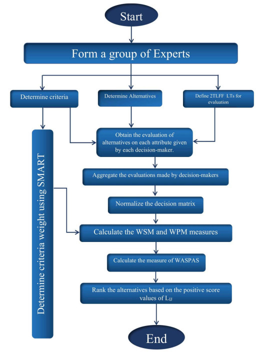
1. We choose a number of DMs who have a complete mastery over the topic.
2. In this step, the DMs define a set of alternatives. The selected DMs list the alternatives that are essential for the evaluation process after fully understanding the problem.
3. Define a set of attributes. The selected DMs list the alternatives that are essential for evaluation process. These attributes are defined with the help of previous studies on the particular subject.
4. In this step, the DM uses the SMART method [60] to determine the weight of each attribute. In this method, the DM is asked to assign 10 points to the least important criterion/criteria. The sum of the points for each criterion is calculated. The final criteria weights are determined by normalization of the sum of points.
5. Define the LTs and corresponding 2TLFFNs. These linguistic terms and corresponding 2TLFFNs are defined by the DMs.
6. Obtain the judgment of the DMs on each attribute in the form of linguistic terms.
7. Convert the linguistic matrices into assessing matrices (AsMs).
8. In this step, the DM can evaluate alternatives using the 2TLFFHWAO and 2TLFFHWGO, i.e., the $ i $th alternative is evaluated by the $ k $th DM on the basis of the $ j $th criteria.
|
$ Qij=(Δ(t3√1−q∏k=1(1−(Δ−1(ˉsϕkij,ϕkij)/t)3)ωk)),Δ(tq∏k=1(Δ−1(ˉsθkij,θkij)/t)ωk)), $
|
(3.1) |
|
$ Qij=(Δ(tm∏k=1(Δ−1(ˉsθkij,θkij)/t)ωj),Δ(t3√1−m∏k=1(1−(Δ−1(ˉsϕkij,ϕkij)/t)3)ωj)). $
|
(3.2) |
9. In this step, if the criterion is a beneficial criterion (BeC), then it does not change, but if it is a non-beneficial criterion (NoC), we take the complement as defined in this Equation 3.3.
|
$ Com(Qij)={(ˉsθ,θ),(ˉsϕ,ϕ)}. $
|
(3.3) |
The normalized decision matrix can be calculated as
|
$ Lkij={(ˉsϕkij,ϕkij),(ˉsθkij,θkij)}={Qijifj∈BeC,Com(Qij)ifj∈NoC. $
|
(3.4) |
10. We calculate the WeSM and WePM measures by using Propositions 2.1 and 2.2 (using $ \gamma = 1 $).
$ L_{ij}^s = 2TLFFHWA(\delta^{1}_{ij}, \delta^{2}_{ij}, \ldots, \delta^{m}_{ij})\\ = \bigoplus^m_{k = 1}(\omega_{j}\otimes L^{k}_{ij}) \\ = \Bigg(\Delta\Bigg(t\sqrt[3]{1-\prod^m_{k = 1}(1-(\Delta^{-1}(\bar{s}_{\phi_{ij}^{k}}, \phi_{ij}^{k})/t)^3)^{\omega_{k}}})\Bigg), \Delta\Bigg(t{\prod^m_{k = 1}(\Delta^{-1}(\bar{s}_{\theta_{ij}^{k}}, \theta_{ij}^{k})/t)^{\omega_{j}}}\Bigg)\Bigg), $
$ L_{ij}^p = 2TLFFHWG(\delta^{1}_{ij}, \delta^{2}_{ij}, \ldots, \delta^{m}_{ij})\\ = \bigotimes^m_{k = 1}(\omega_{j}\otimes L^{k}_{ij}) \\ = \Bigg(\Delta\Bigg(t{\prod^m_{k = 1}(\Delta^{-1}(\bar{s}_{\theta_{ij}^{k}}, \theta_{ij}^{k})/t)^{\omega_{j}}}\Bigg), \Delta\Bigg(t\sqrt[3]{1-\prod^m_{k = 1}{(1-(\Delta^{-1}(\bar{s}_{\phi_{ij}^{k}}, \phi_{ij}^{k})/t)^3)^{\omega_{j}}}}\Bigg)\Bigg). $
Now calculate the measure of WASPAS by using Equation 3.5.
|
$ Lij=τLsij⊕(1−τ)Lpij. $
|
(3.5) |
$ $Calculate the ranking of the alternatives using the formula given below, where $ \dot{S}^{p}(\delta_1) $ represents the positive score function and $ \dot{S}(\delta_1) $ represents the score function.
|
$ ˙Sp(δ1)=1+˙S(δ1). $
|
(3.6) |
In this section, we extend the WASPAS method with the 2TLFFHWA operator, 2TLFFHWG operator, WeSM and WePM under the 2TLFF environment.
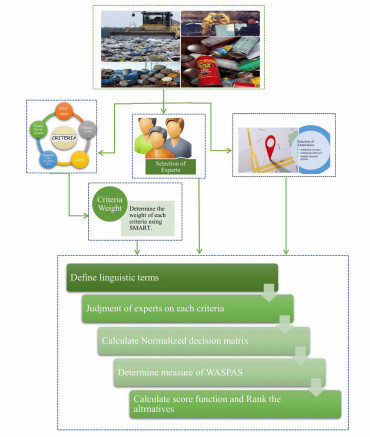
Example 4.1 (SWDLS problem). In many cities of the United Kingdom, manufacturing companies are trendy and a key concern. Manchester is a city of the UK with a lot of cultures. There are many public and private manufacturing companies in Manchester. These manufacturing plants produce a lot of solid waste and pollution. Solid waste can cause various diseases in humansuch as bacillary dysentery, amoebic dysentery, cholera, jaundice, gastero, enteric diseases, endemic typhus, salmonellosis, trichinosis, diarrhea, plague, etc. Nowadays, disposal of this type of waste is a big issue. Consequently, finding the best place to dispose of such waste is an essential job of manufacturing organizations. We have used three main manufacturing companies of Manchester namely, Manchester manufacturing group, Automation technology and Iceland manufacturing limited to choose the best location for disposal of their solid waste. The waste management procedures of the above-mentioned manufacturing plants were monitored and we collected the information about collection, storage and disposal of their solid waste. The total waste bags produced were recorded. The weights of each waste bag were also recorded from each company. Although these companies have proper disposal system, due to continued enlargement and increasing product demand of these companies, the administration is supposed to build a proper waste disposal location. The aim of this research article is to introduce MAGDM methodology to select the best location for the disposal of waste.
We have selected the attributes and alternatives on the basis of the DM's opinion, research articles, case studies, etc. A flowchart of the application using the WASPAS method is shown in Figure 3.
A. Solution of SWDLS problem using the extended WASPAS method with the 2TLFFHWAO
We solve the SWDLS problem by using the extended WASPAS measure with the 2TLFFHWGO which is defined in 2.1.
1. We have selected three DMs ($ E_1 $, $ E_2 $ and $ E_3 $). The first DM is the plant manager, second is the factory engineer and third is the production manager. The collective opinions of all these DMs were used in decision-making. The WV of DMs the (0.2, 0.5, 0.3).
2. The DMs thoroughly studied and checked out the history of methods to dispose waste. On the basis of their study and after screening the list of possible landfill locations, they obtained a set of 4 alternatives ($ W_1 $ to $ W_4 $). The following four alternatives have been selected as listed in Table 2.
| Alternatives | Site name |
| Astley sand and aggregated limited ($ W_1 $) | Morleys quarry |
| Augean north limited ($ W_2 $) | Marks Quarry Landfill site |
| Augean west limited ($ W_3 $) | Port Clarence non-hazardous landfill site |
| Augean south limited ($ W_4 $) | East Northants resource management facility |
DownLoad:
CSV
3. For defining the criteria and the DMs studied research articles, literature and conducted surveys. Following five attributes have been selected as listed in Table 3.
| Attribute | Type | Definition |
| Distance ($ T_1 $) | benefit | Distance from populated areas |
| Disease vector ($ T_2 $) | cost | Breeding of vectors in (e.g., rats, mosquitos) in landfill |
| Cost ($ T_3 $) | Cost | Land price, transportation cost and employee salary |
| Future development ($ T_4 $) | Benefit | possibility of development of land in future |
| Geographical circumstances ($ T_5 $) | Benefit | study of natural features of Earth's surface |
DownLoad:
CSV
4. To calculate criteria weights, we used the SMART method [60]. The results are recorded in Table 4.
| Attribute | Type | $ E_1 $ | $ E_2 $ | $ E_3 $ | Sum | $ w_j $ |
| Distance ($ T_1 $) | benefit | 80 | 70 | 85 | 235 | 0.23 |
| Disease vector ($ T_2 $) | cost | 40 | 30 | 60 | 130 | 0.13 |
| Cost ($ T_3 $) | cost | 90 | 90 | 80 | 260 | 0.26 |
| Future development ($ T_4 $) | benefit | 70 | 60 | 50 | 180 | 0.18 |
| Geographical circumstances ($ T_5 $) | benefit | 65 | 50 | 85 | 200 | 0.20 |
DownLoad:
CSV
5. Now we define LT for the 2TLFFNs which are given in Table 5.
| LV | 2TLFFNs |
| Very low ($ \ddot{VL} $) | $ \{(\bar{s}_0, 0), (\bar{s}_6, 0)\} $ |
| Low ($ \ddot{L} $) | $ \{(\bar{s}_1, 0), (\bar{s}_5, 0)\} $ |
| Medium Low ($ \ddot{ML} $) | $ \{(\bar{s}_2, 0), (\bar{s}_4, 0)\} $ |
| Medium ($ \ddot{M} $) | $ \{(\bar{s}_3, 0), (\bar{s}_3, 0)\} $ |
| Medium High ($ \ddot{MH} $) | $ \{(\bar{s}_4, 0), (\bar{s}_2, 0)\} $ |
| High ($ \ddot{H} $) | $ \{(\bar{s}_5, 0), (\bar{s}_1, 0)\} $ |
| Very High ($ \ddot{VH} $) | $ \{(\bar{s}_6, 0), (\bar{s}_0, 0)\} $ |
DownLoad:
CSV
6. Each DM judges the alternatives on each criteria. The results are given in Table 6.
| DMs | Sites | $ T_1 $ | $ T_2 $ | $ T_3 $ | $ T_4 $ | $ T_5 $ |
| $ E_1 $ | $ W_1 $ | $ \ddot{H} $ | $ \ddot{H} $ | $ \ddot{L} $ | $ \ddot{L} $ | $ \ddot{MH} $ |
| $ W_2 $ | $ \ddot{M} $ | $ \ddot{ML} $ | $ \ddot{MH} $ | $ \ddot{L} $ | $ \ddot{ML} $ | |
| $ W_3 $ | $ \ddot{L} $ | $ \ddot{H} $ | $ \ddot{H} $ | $ \ddot{M} $ | $ \ddot{VH} $ | |
| $ W_4 $ | $ \ddot{L} $ | $ \ddot{MH} $ | $ \ddot{M} $ | $ \ddot{H} $ | $ \ddot{L} $ | |
| $ E_2 $ | $ W_1 $ | $ \ddot{H} $ | $ \ddot{H} $ | $ \ddot{L} $ | $ \ddot{M} $ | $ \ddot{M} $ |
| $ W_2 $ | $ \ddot{M} $ | $ \ddot{M} $ | $ \ddot{MH} $ | $ \ddot{H} $ | $ \ddot{H} $ | |
| $ W_3 $ | $ \ddot{VH} $ | $ \ddot{H} $ | $ \ddot{MH} $ | $ \ddot{M} $ | $ \ddot{VH} $ | |
| $ W_4 $ | $ \ddot{L} $ | $ \ddot{L} $ | $ \ddot{M} $ | $ \ddot{MH} $ | $ \ddot{L} $ | |
| $ E_3 $ | $ W_1 $ | $ \ddot{H} $ | $ \ddot{VH} $ | $ \ddot{H} $ | $ \ddot{MH} $ | $ \ddot{MH} $ |
| $ W_2 $ | $ \ddot{M} $ | $ \ddot{L} $ | $ \ddot{L} $ | $ \ddot{L} $ | $ \ddot{ML} $ | |
| $ W_3 $ | $ \ddot{H} $ | $ \ddot{H} $ | $ \ddot{H} $ | $ \ddot{M} $ | $ \ddot{MH} $ | |
| $ W_4 $ | $ \ddot{H} $ | $ \ddot{H} $ | $ \ddot{M} $ | $ \ddot{H} $ | $ \ddot{H} $ |
DownLoad:
CSV
7. We convert the LAM given in Table 6 into AsMs. The outcomes are given in Table 7.
| DMs | Sites | $ T_1 $ | $ T_2 $ | $ T_3 $ | $ T_4 $ | $ T_5 $ |
| $ E_1 $ | $ W_1 $ | $ \{(\bar{s}_5, 0), (\bar{s}_1, 0)\} $ | $ \{(\bar{s}_5, 0), (\bar{s}_1, 0)\} $ | $ \{(\bar{s}_1, 0), (\bar{s}_5, 0)\} $ | $ \{(\bar{s}_1, 0), (\bar{s}_5, 0)\} $ | $ \{(\bar{s}_4, 0), (\bar{s}_2, 0)\} $ |
| $ W_2 $ | $ \{(\bar{s}_3, 0), (\bar{s}_3, 0)\} $ | $ \{(\bar{s}_2, 0), (\bar{s}_4, 0)\} $ | $ \{(\bar{s}_1, 0), (\bar{s}_5, 0)\} $ | $ \{(\bar{s}_1, 0), (\bar{s}_5, 0)\} $ | $ \{(\bar{s}_2, 0), (\bar{s}_4, 0)\} $ | |
| $ W_3 $ | $ \{(\bar{s}_1, 0), (\bar{s}_5, 0)\} $ | $ \{(\bar{s}_5, 0), (\bar{s}_1, 0)\} $ | $ \{(\bar{s}_5, 0), (\bar{s}_1, 0)\} $ | $ \{(\bar{s}_3, 0), (\bar{s}_3, 0)\} $ | $ \{(\bar{s}_6, 0), (\bar{s}_0, 0)\} $ | |
| $ W_4 $ | $ \{(\bar{s}_1, 0), (\bar{s}_5, 0)\} $ | $ \{(\bar{s}_4, 0), (\bar{s}_2, 0)\} $ | $ \{(\bar{s}_3, 0), (\bar{s}_3, 0)\} $ | $ \{(\bar{s}_5, 0), (\bar{s}_1, 0)\} $ | $ \{(\bar{s}_1, 0), (\bar{s}_5, 0)\} $ | |
| $ E_2 $ | $ W_1 $ | $ \{(\bar{s}_5, 0), (\bar{s}_1, 0)\} $ | $ \{(\bar{s}_5, 0), (\bar{s}_1, 0)\} $ | $ \{(\bar{s}_1, 0), (\bar{s}_5, 0)\} $ | $ \{(\bar{s}_3, 0), (\bar{s}_3, 0)\} $ | $ \{(\bar{s}_3, 0), (\bar{s}_3, 0)\} $ |
| $ W_2 $ | $ \{(\bar{s}_3, 0), (\bar{s}_3, 0)\} $ | $ \{(\bar{s}_3, 0), (\bar{s}_3, 0)\} $ | $ \{(\bar{s}_4, 0), (\bar{s}_2, 0)\} $ | $ \{(\bar{s}_5, 0), (\bar{s}_1, 0)\} $ | $ \{(\bar{s}_5, 0), (\bar{s}_1, 0)\} $ | |
| $ W_3 $ | $ \{(\bar{s}_6, 0), (\bar{s}_0, 0)\} $ | $ \{(\bar{s}_5, 0), (\bar{s}_1, 0)\} $ | $ \{(\bar{s}_4, 0), (\bar{s}_2, 0)\} $ | $ \{(\bar{s}_3, 0), (\bar{s}_3, 0)\} $ | $ \{(\bar{s}_6, 0), (\bar{s}_0, 0)\} $ | |
| $ W_4 $ | $ \{(\bar{s}_1, 0), (\bar{s}_5, 0)\} $ | $ \{(\bar{s}_1, 0), (\bar{s}_5, 0)\} $ | $ \{(\bar{s}_3, 0), (\bar{s}_3, 0)\} $ | $ \{(\bar{s}_4, 0), (\bar{s}_2, 0)\} $ | $ \{(\bar{s}_0, 0), (\bar{s}_6, 0)\} $ | |
| $ E_3 $ | $ W_1 $ | $ \{(\bar{s}_5, 0), (\bar{s}_1, 0)\} $ | $ \{(\bar{s}_6, 0), (\bar{s}_0, 0)\} $ | $ \{(\bar{s}_5, 0), (\bar{s}_1, 0)\} $ | $ \{(\bar{s}_4, 0), (\bar{s}_2, 0)\} $ | $ \{(\bar{s}_4, 0), (\bar{s}_2, 0)\} $ |
| $ W_2 $ | $ \{(\bar{s}_3, 0), (\bar{s}_3, 0)\} $ | $ \{(\bar{s}_1, 0), (\bar{s}_5, 0)\} $ | $ \{(\bar{s}_1, 0), (\bar{s}_5, 0)\} $ | $ \{(\bar{s}_1, 0), (\bar{s}_5, 0)\} $ | $ \{(\bar{s}_2, 0), (\bar{s}_4, 0)\} $ | |
| $ W_3 $ | $ \{(\bar{s}_5, 0), (\bar{s}_1, 0)\} $ | $ \{(\bar{s}_5, 0), (\bar{s}_1, 0)\} $ | $ \{(\bar{s}_5, 0), (\bar{s}_1, 0)\} $ | $ \{(\bar{s}_3, 0), (\bar{s}_3, 0)\} $ | $ \{(\bar{s}_4, 0), (\bar{s}_2, 0)\} $ | |
| $ W_4 $ | $ \{(\bar{s}_5, 0), (\bar{s}_1, 0)\} $ | $ \{(\bar{s}_5, 0), (\bar{s}_1, 0)\} $ | $ \{(\bar{s}_3, 0), (\bar{s}_3, 0)\} $ | $ \{(\bar{s}_5, 0), (\bar{s}_1, 0)\} $ | $ \{(\bar{s}_5, 0), (\bar{s}_1, 0)\} $ |
DownLoad:
CSV
8. The AsMs were aggregated based on Equation 3.1. Then we obtained $ Q_{ij} $. The results are recorded in Table 8.
| Sites | $ T_1 $ | $ T_2 $ | $ T_3 $ | $ T_4 $ | $ T_5 $ |
| $ W_1 $ | $ \{(\bar{s}_5, 0), (\bar{s}_1, 0)\} $ | $ \{(\bar{s}_6, 0), (\bar{s}_0, 0)\} $ | $ \{(\bar{s}_4, -0.33), (\bar{s}_3, 0.5)\} $ | $ \{(\bar{s}_3, 0.25), (\bar{s}_3, -0.05)\} $ | $ \{(\bar{s}_4, -0.40), (\bar{s}_2, 0.44)\} $ |
| $ W_2 $ | $ \{(\bar{s}_3, 0), (\bar{s}_3, 0)\} $ | $ \{(\bar{s}_2, 0.5), (\bar{s}_4, -0.29)\} $ | $ \{(\bar{s}_4, -0.38), (\bar{s}_3, -0.63)\} $ | $ \{(\bar{s}_4, 0.23), (\bar{s}_2, 0.44)\} $ | $ \{(\bar{s}_4, 0.28), (\bar{s}_2, 0)\} $ |
| $ W_3 $ | $ \{(\bar{s}_6, 0), (\bar{s}_0, 0)\} $ | $ \{(\bar{s}_5, 0), (\bar{s}_1, 0)\} $ | $ \{(\bar{s}_5, -0.38), (\bar{s}_1, 0.41)\} $ | $ \{(\bar{s}_3, 0), (\bar{s}_3, 0)\} $ | $ \{(\bar{s}_6, 0), (\bar{s}_0, 0)\} $ |
| $ W_4 $ | $ \{(\bar{s}_4, -0.33), (\bar{s}_3, 0.50)\} $ | $ \{(\bar{s}_4, -0.06), (\bar{s}_3, -0.43)\} $ | $ \{(\bar{s}_3, 0), (\bar{s}_3, 0)\} $ | $ \{(\bar{s}_5, -0.38), (\bar{s}_1, 0.41)\} $ | $ \{(\bar{s}_4, -0.32), (\bar{s}_3, 0.37)\} $ |
DownLoad:
CSV
9. The calculated results of the normalized decision matrix using Equation 3.4 are given in Table 9.
| Sites | $ T_1 $ | $ T_2 $ | $ T_3 $ | $ T_4 $ | $ T_5 $ |
| $ W_1 $ | $ \{(\bar{s}_6, 0), (\bar{s}_0, 0)\} $ | $ \{(\bar{s}_0, 0), (\bar{s}_6, 0)\} $ | $ \{(\bar{s}_3, 0.5), (\bar{s}_4, -0.33)\} $ | $ \{(\bar{s}_3, 0.25), (\bar{s}_3, -0.05)\} $ | $ \{(\bar{s}_4, -0.40), (\bar{s}_2, 0.44)\} $ |
| $ W_2 $ | $ \{(\bar{s}_3, 0), (\bar{s}_3, 0)\} $ | $ \{(\bar{s}_4, -0.29), (\bar{s}_2, 0.5)\} $ | $ \{(\bar{s}_3, -0.63), (\bar{s}_4, -0.38)\} $ | $ \{(\bar{s}_4, 0.23), (\bar{s}_2, 0.44)\} $ | $ \{(\bar{s}_4, 0.28), (\bar{s}_2, 0)\} $ |
| $ W_3 $ | $ \{(\bar{s}_6, 0), (\bar{s}_0, 0)\} $ | $ \{(\bar{s}_1, 0), (\bar{s}_5, 0) \} $ | $ \{(\bar{s}_1, 0.41), (\bar{s}_5, -0.38)\} $ | $ \{(\bar{s}_3, 0), (\bar{s}_3, 0)\} $ | $ \{(\bar{s}_6, 0), (\bar{s}_0, 0)\} $ |
| $ W_4 $ | $ \{(\bar{s}_4, -0.33), (\bar{s}_3, 0.50)\} $ | $ \{(\bar{s}_3, -0.43), (\bar{s}_4, -0.06)\} $ | $ \{(\bar{s}_3, 0), (\bar{s}_3, 0)\} $ | $ \{(\bar{s}_5, -0.38), (\bar{s}_1, 0.41)\} $ | $ \{(\bar{s}_4, -0.32), (\bar{s}_3, 0.37)\} $ |
DownLoad:
CSV
10. The calculated result of the WeSM, WePM and WASPAS measures by using the following equations and results are recorded in Table 10. $ L_{ij}^s = 2TLFFHWA(\delta^{1}_{ij}, \delta^{2}_{ij}, \ldots, \delta^{m}_{ij}) $
$ = \bigoplus^m_{k = 1}(\omega_{j}\otimes L^{k}_{ij}) \\ = \Bigg(\Delta\Bigg(t\sqrt[3]{1-\prod^m_{k = 1}(1-(\Delta^{-1}(\bar{s}_{\phi_{ij}^{k}}, \phi_{ij}^{k})/t)^3)^{\omega_{k}}})\Bigg), \Delta\Bigg(t{\prod^m_{k = 1}(\Delta^{-1}(\bar{s}_{\theta_{ij}^{k}}, \theta_{ij}^{k})/t)^{\omega_{j}}}\Bigg)\Bigg), \\ L_{ij}^p = 2TLFFHWG(\delta^{1}_{ij}, \delta^{2}_{ij}, \ldots, \delta^{m}_{ij})\\ = \bigotimes^m_{k = 1}(\omega_{j}\otimes L^{k}_{ij}) \\ = \Bigg(\Delta\Bigg(t{\prod^m_{k = 1}(\Delta^{-1}(\bar{s}_{\theta_{ij}^{k}}, \theta_{ij}^{k})/t)^{\omega_{j}}}\Bigg), \Delta\Bigg(t\sqrt[3]{1-\prod^m_{k = 1}{(1-(\Delta^{-1}(\bar{s}_{\phi_{ij}^{k}}, \phi_{ij}^{k})/t)^3)^{\omega_{j}}}}\Bigg)\Bigg). $
| Sites | $ L_{ij}^{s} $ | $ L_{ij}^p $ | $ L_{ij} $ |
| $ W_1 $ | $ \{(\bar{s}_6, 0), (\bar{s}_0, 0)\} $ | $ \{(\bar{s}_4, 0.26), (\bar{s}_3, -0.30)\} $ | $ \{(\bar{s}_6, 0), (\bar{s}_0, 0.01)\} $ |
| $ W_2 $ | $ \{(\bar{s}_4, -0.28), (\bar{s}_3, -0.35)\} $ | $ \{(\bar{s}_4, -0.48), (\bar{s}_3, -0.18)\} $ | $ \{(\bar{s}_4, -0.37), (\bar{s}_0, 0.01)\} $ |
| $ W_3 $ | $ \{(\bar{s}_6, 0), (\bar{s}_0, 0)\} $ | $ \{(\bar{s}_5, -0.16), (\bar{s}_2, -0.18)\} $ | $ \{(\bar{s}_6, 0), (\bar{s}_0, 0)\} $ |
| $ W_4 $ | $ \{(\bar{s}_4, -0.18), (\bar{s}_3, -0.32)\} $ | $ \{(\bar{s}_4, -0.33), (\bar{s}_3, 0.03)\} $ | $ \{(\bar{s}_3, -0.25), (\bar{s}_0, 0.05)\} $ |
DownLoad:
CSV
11. The calculated results of the score function of $ L_{ij} $ based on Definition 2.7 and the ranking of locations are given in Table 11.
| Sites | $ \dot{S}(L_{ij}) $ | Ranking |
| $ W_1 $ | 5.999 | 2 |
| $ W_2 $ | 1.3208 | 4 |
| $ W_3 $ | 6 | 1 |
| $ W_4 $ | 1.45859 | 3 |
DownLoad:
CSV
From Table 11, we can deduce that $ W_3 > W_1 > W_4 > W_2 $. Thus, $ W_3 $ is the best location to dispose of the solid waste.
B. Solution of SWDLS problem using the extended WASPAS method with the 2TLFFHWGO
We solved the SWDLS problem by the extended WASPAS measure with the 2TLFFHWGO which is defined in 2.2.
1. The AsMs were aggregated based on Equation 3.2. The results are recorded in Table 12.
| Sites | $ T_1 $ | $ T_2 $ | $ T_3 $ | $ T_4 $ | $ T_5 $ |
| $ W_1 $ | $ \{(\bar{s}_5, 0.47), (\bar{s}_1, -0.20)\} $ | $ \{(\bar{s}_5, 0.28), (\bar{s}_1, -0.11)\} $ | $ \{(\bar{s}_2, -0.38), (\bar{s}_5, -0.38)\} $ | $ \{(\bar{s}_3, -0.37), (\bar{s}_4, -0.36)\} $ | $ \{(\bar{s}_3, 0.46), (\bar{s}_3, -0.39)\} $ |
| $ W_2 $ | $ \{(\bar{s}_3, 0), (\bar{s}_3, 0)\} $ | $ \{(\bar{s}_2, -0.01), (\bar{s}_4, 0.13)\} $ | $ \{(\bar{s}_3, -0.36), (\bar{s}_4, -0.22)\} $ | $ \{(\bar{s}_2, 0.23), (\bar{s}_4, 0.23)\} $ | $ \{(\bar{s}_3, 0.16), (\bar{s}_3, 0.27)\} $ |
| $ W_3 $ | $ \{(\bar{s}_4, -0.04), (\bar{s}_3, 0.25)\} $ | $ \{(\bar{s}_5, 0), (\bar{s}_1, 0)\} $ | $ \{(\bar{s}_4, 0.47), (\bar{s}_2, -0.34)\} $ | $ \{(\bar{s}_3, 0), (\bar{s}_3, 0)\} $ | $ \{(\bar{s}_5, 0.31), (\bar{s}_1, 0.34)\} $ |
| $ W_4 $ | $ \{(\bar{s}_2, -0.38), (\bar{s}_5, -0.39)\} $ | $ \{(\bar{s}_2, 0.13), (\bar{s}_4, 0.25)\} $ | $ \{(\bar{s}_3, 0), (\bar{s}_3, 0)\} $ | $ \{(\bar{s}_4, 0.47), (\bar{s}_2, -0.34)\} $ | $ \{(\bar{s}_2, -0.38), (\bar{s}_5, -0.38)\} $ |
DownLoad:
CSV
2. The calculated results of the normalized decision matrix are given in Table 13.
| Sites | $ T_1 $ | $ T_2 $ | $ T_3 $ | $ T_4 $ | $ T_5 $ |
| $ W_1 $ | $ \{(\bar{s}_5, 0.47), (\bar{s}_1, -0.20)\} $ | $ \{ (\bar{s}_1, -0.11), (\bar{s}_5, 0.28)\} $ | $ \{(\bar{s}_5, -0.38), (\bar{s}_2, -0.38) \} $ | $ \{(\bar{s}_3, -0.37), (\bar{s}_4, -0.36)\} $ | $ \{(\bar{s}_3, 0.46), (\bar{s}_3, -0.39)\} $ |
| $ W_2 $ | $ \{(\bar{s}_3, 0), (\bar{s}_3, 0)\} $ | $ \{ (\bar{s}_4, 0.13), (\bar{s}_2, -0.01)\} $ | $ \{(\bar{s}_4, -0.22), (\bar{s}_3, -0.36) \} $ | $ \{(\bar{s}_2, 0.23), (\bar{s}_4, 0.23)\} $ | $ \{(\bar{s}_3, 0.16), (\bar{s}_3, 0.27)\} $ |
| $ W_3 $ | $ \{(\bar{s}_4, -0.04), (\bar{s}_3, 0.25)\} $ | $ \{ (\bar{s}_1, 0), (\bar{s}_5, 0)\} $ | $ \{ (\bar{s}_2, -0.34), (\bar{s}_4, 0.47)\} $ | $ \{(\bar{s}_3, 0), (\bar{s}_3, 0)\} $ | $ \{(\bar{s}_5, 0.31), (\bar{s}_1, 0.34)\} $ |
| $ W_4 $ | $ \{(\bar{s}_2, -0.38), (\bar{s}_5, -0.39)\} $ | $ \{ (\bar{s}_4, 0.25), (\bar{s}_2, 0.13)\} $ | $ \{(\bar{s}_3, 0), (\bar{s}_3, 0)\} $ | $ \{(\bar{s}_4, 0.47), (\bar{s}_2, -0.34)\} $ | $ \{(\bar{s}_2, -0.38), (\bar{s}_5, -0.39)\} $ |
DownLoad:
CSV
3. We calculated the WeSM, WePM and WASPAS measures by the Definition 2.9 with $ \gamma = 1 $. The results are recorded in Table 14.
| Sites | $ L_{ij}^{s} $ | $ L_{ij}^p $ | $ L_{ij} $ |
| $ W_1 $ | $ \{(\bar{s}_4, -0.29), (\bar{s}_0, 0.28)\} $ | $ \{(\bar{s}_3, -0.45), (\bar{s}_0, 0.44)\} $ | $ \{(\bar{s}_4, -0.01), (\bar{s}_0, 0.021)\} $ |
| $ W_2 $ | $ \{(\bar{s}_2, 0.19), (\bar{s}_0, 0.40)\} $ | $ \{(\bar{s}_2, 0.1), (\bar{s}_0, 0.48)\} $ | $ \{(\bar{s}_3, -0.31), (\bar{s}_0, 0.03)\} $ |
| $ W_3 $ | $ \{(\bar{s}_4, -0.2), (\bar{s}_0, 0.106)\} $ | $ \{(\bar{s}_3.0.49), (\bar{s}_0, 0.26)\} $ | $ \{(\bar{s}_4, 0.43), (\bar{s}_0, 0.004)\} $ |
| $ W_4 $ | $ \{(\bar{s}_2, 0.47), (\bar{s}_1, 0)\} $ | $ \{(\bar{s}_2, -0.12), (\bar{s}_1, 0)\} $ | $ \{(\bar{s}_3, -0.22), (\bar{s}_0, 0.16)\} $ |
DownLoad:
CSV
4. The calculated results of the score function of $ L_{ij} $ using Definition 2.7 and the ranking of locations are given in Table 15. From Table 15, we conclude that $ W_3 > W_1 > W_4 > W_2 $. Thus, $ W_3 $ is the best location to dispose of the solid waste of manufacturing plants.
| Sites | $ \dot{S}(L_{ij}) $ | Ranking |
| $ W_1 $ | 1.7757 | 2 |
| $ W_2 $ | 0.53986 | 4 |
| $ W_3 $ | 2.41718 | 1 |
| $ W_4 $ | 0.59495 | 3 |
DownLoad:
CSV
C. Solution of SWDLS problem using the extended WeSM with the 2TLFFNs
We solved the SWDLS problem by the extended WeSM measure with 2TLFFNs. In the WeSM, we put $ \tau = 1 $ in Equation 3.5. The results obtained are shown in Tables 16 and 17.
| Sites | $ L_{ij}^{s} $ | $ L_{ij}^p $ | $ L_{ij} $ |
| $ W_1 $ | $ \{(\bar{s}_6, 0), (\bar{s}_0, 0)\} $ | $ \{(\bar{s}_4, 0.26), (\bar{s}_3, -0.30)\} $ | $ \{(\bar{s}_6, 0), (\bar{s}_0, 0.01)\} $ |
| $ W_2 $ | $ \{(\bar{s}_4, -0.28), (\bar{s}_3, -0.35)\} $ | $ \{(\bar{s}_4, -0.48), (\bar{s}_3, -0.18)\} $ | $ \{(\bar{s}_4, -0.28), (\bar{s}_3, -0.35)\} $ |
| $ W_3 $ | $ \{(\bar{s}_6, 0), (\bar{s}_0, 0)\} $ | $ \{(\bar{s}_5, -0.16), (\bar{s}_2, -0.18)\} $ | $ \{(\bar{s}_6, 0), (\bar{s}_0, 0)\} $ |
| $ W_4 $ | $ \{(\bar{s}_4, -0.18), (\bar{s}_3, -0.32)\} $ | $ \{(\bar{s}_4, -0.33), (\bar{s}_3, 0.03)\} $ | $ \{(\bar{s}_4, -0.18), (\bar{s}_3, -0.32)\} $ |
DownLoad:
CSV
| Sites | $ \dot{S}(L_{ij}) $ | Ranking |
| $ W_1 $ | 6 | 1 |
| $ W_2 $ | 0.9161 | 3 |
| $ W_3 $ | 6 | 1 |
| $ W_4 $ | 0.9885 | 2 |
DownLoad:
CSV
From Table 17, we conclude that $ W_3 = W_1 > W_4 > W_2 $. Thus, $ W_3 $ and $ W_1 $ are the best locations to dispose of the solid waste of manufacturing plants.
D. Solution of SWDLS problem using the extended WePM with the 2TLFFNs
Now we solve the SWDLS problem by the extended WePM with 2TLFFNs. In the WePM, we put $ \tau = 0 $ in Equation 3.5. The results obtained are shown in Tables 18 and 19.
| Sites | $ L_{ij}^{s} $ | $ L_{ij}^p $ | $ L_{ij} $ |
| $ W_1 $ | $ \{(\bar{s}_6, 0), (\bar{s}_0, 0)\} $ | $ \{(\bar{s}_4, 0.26), (\bar{s}_3, -0.30)\} $ | $ \{(\bar{s}_4, 0.26), (\bar{s}_3, -0.30)\} $ |
| $ W_2 $ | $ \{(\bar{s}_4, -0.28), (\bar{s}_3, -0.35)\} $ | $ \{(\bar{s}_4, -0.48), (\bar{s}_3, -0.18)\} $ | $ \{(\bar{s}_4, -0.48), (\bar{s}_3, -0.18)\} $ |
| $ W_3 $ | $ \{(\bar{s}_6, 0), (\bar{s}_0, 0)\} $ | $ \{(\bar{s}_5, -0.16), (\bar{s}_2, -0.18)\} $ | $ \{(\bar{s}_5, -0.16), (\bar{s}_2, -0.18)\} $ |
| $ W_4 $ | $ \{(\bar{s}_4, -0.18), (\bar{s}_3, -0.32)\} $ | $ \{(\bar{s}_5, -0.16), (\bar{s}_2, -0.18)\} $ | $ \{(\bar{s}_5, -0.16), (\bar{s}_2, -0.18)\} $ |
DownLoad:
CSV
| Sites | $ \dot{S}(L_{ij}) $ | Ranking |
| $ W_1 $ | 1.6181 | 2 |
| $ W_2 $ | 0.58762 | 4 |
| $ W_3 $ | 2.96668 | 1 |
| $ W_4 $ | 0.59008 | 3 |
DownLoad:
CSV
From Table 19, we can infer that $ W_3 > W_1 > W_4 > W_2 $. Thus, $ W_3 $ is the best location to dispose of the solid waste of manufacturing plants.
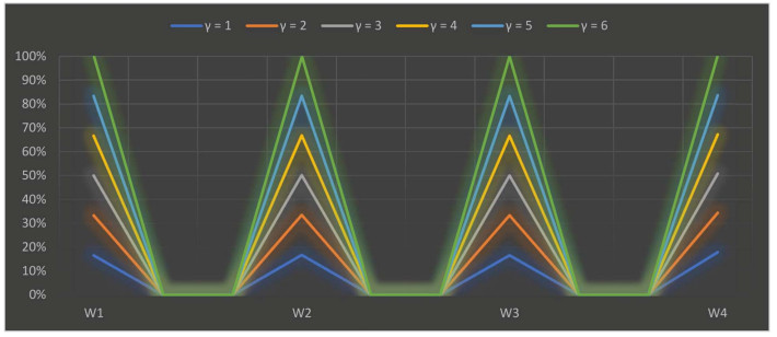
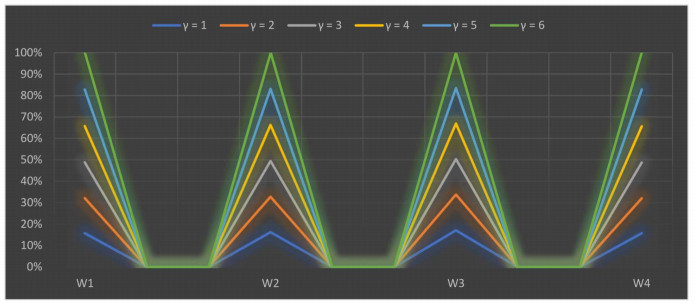
The parameter $ \gamma $ is used in our research study to explain the interdependency between distinct quantifiable attributes. Various numerical values of the parameter $ \gamma $ illustrate the various decision-making possibilities and circumstances. We assigned numerical values from $ 1 $ to $ 6 $ to $ \gamma $ the results are shown in Tables 20 and 21. The scoring values of each selected alternative varied depending on the crisp value of the parameter, but the derived results are roughly the same. When we allocated distinguishable numerical values to the parameter $ \gamma $, the best alternative is $ O_3 $ for the SWDLS problem solved with the extended 2TLFF-WASPAS method using two different operators, i.e., the 2TLFFHWA operator and 2TLFFHWG operator. We can also summarize from the appraisal scoring results as shown in Tables 20 and 21 that the 2TLFFHWA and 2TLFFHWG operators proposed in this research study are the best approaches to summarize aggregated 2TLFF information. A graph of the ranking results of SWDLS by the 2TLFFHWAO using different values of $ \gamma $ is shown in Figure 4.
| Parameter | $ \dot{S}(W_1) $ | $ \dot{S}(W_2) $ | $ \dot{S}(W_3) $ | $ \dot{S}(W_4) $ | Ranking |
| $ \gamma=1 $ | $ (\bar{s}_6, -0.0001) $ | $ (\bar{s}_4, -0.29) $ | $ (\bar{s}_6, 0) $ | $ (\bar{s}_4, -0.34) $ | $ W_3 > W_1 > W_2 > W_4 $ |
| $ \gamma=2 $ | $ (\bar{s}_6, -0.00001) $ | $ (\bar{s}_4, -0.30) $ | $ (\bar{s}_6, 0) $ | $ (\bar{s}_3, 0.34) $ | $ W_3 > W_1 > W_2 > W_4 $ |
| $ \gamma=3 $ | $ (\bar{s}_6, -0.00001) $ | $ (\bar{s}_4, -0.31) $ | $ (\bar{s}_6, 0) $ | $ (\bar{s}_3, 0.41) $ | $ W_3 > W_1 > W_2 > W_4 $ |
| $ \gamma=4 $ | $ (\bar{s}_6, -0.000001) $ | $ (\bar{s}_3, 0.32) $ | $ (\bar{s}_6, 0) $ | $ (\bar{s}_3, 0.33) $ | $ W_3 > W_1 > W_2 > W_4 $ |
| $ \gamma=5 $ | $ (\bar{s}_6, -0.000001) $ | $ (\bar{s}_3, 0.33) $ | $ (\bar{s}_6, 0) $ | $ (\bar{s}_3, 0.33) $ | $ W_3 > W_1 > W_2 > W_4 $ |
| $ \gamma=6 $ | $ (\bar{s}_6, -0.000001) $ | $ (\bar{s}_3, 0.34) $ | $ (\bar{s}_6, 0) $ | $ (\bar{s}_3, 0.33) $ | $ W_3 > W_1 > W_2 > W_4 $ |
DownLoad:
CSV
| Parameter | $ \dot{S}(W_1) $ | $ \dot{S}(W_2) $ | $ \dot{S}(W_3) $ | $ \dot{S}(W_4) $ | Ranking |
| $ \gamma=1 $ | $ (\bar{s}_2, 0.25) $ | $ (\bar{s}_2, 0.12) $ | $ (\bar{s}_3, -0.08) $ | $ (\bar{s}_2, -0.13) $ | $ W_3 > W_1 > W_2 > W_4 $ |
| $ \gamma=2 $ | $ (\bar{s}_2, 0.32) $ | $ (\bar{s}_2, 0.15) $ | $ (\bar{s}_3, -0.17) $ | $ (\bar{s}_2, -0.06) $ | $ W_3 > W_1 > W_2 > W_4 $ |
| $ \gamma=3 $ | $ (\bar{s}_2, 0.37) $ | $ (\bar{s}_2, 0.17) $ | $ (\bar{s}_3, -0.19) $ | $ (\bar{s}_2, -0.04) $ | $ W_3 > W_1 > W_2 > W_4 $ |
| $ \gamma=4 $ | $ (\bar{s}_2, 0.40) $ | $ (\bar{s}_2, 0.18) $ | $ (\bar{s}_3, -0.19) $ | $ (\bar{s}_2, 0) $ | $ W_3 > W_1 > W_2 > W_4 $ |
| $ \gamma=5 $ | $ (\bar{s}_2, 0.43) $ | $ (\bar{s}_2, 0.19) $ | $ (\bar{s}_3, -0.19) $ | $ (\bar{s}_2, 0.03) $ | $ W_3 > W_1 > W_2 > W_4 $ |
| $ \gamma=6 $ | $ (\bar{s}_2, 0.45) $ | $ (\bar{s}_2, 0.19) $ | $ (\bar{s}_3, -0.19) $ | $ (\bar{s}_2, 0.05) $ | $ W_3 > W_1 > W_2 > W_4 $ |
DownLoad:
CSV
A graph of the ranking results of SWDLS by the 2TLFFHWGO using different values of $ \gamma $ is shown in Figure 5.
We solved the problem of SWDLS using the CODAS method for 2TLPFNs [61].
1. We converted the linguistic assessing matrices which are given in Table 6, into assessing matrices. The outcomes are given in Tables 22, 23 and 24.
| Sites | $ T_1 $ | $ T_2 $ | $ T_3 $ | $ T_4 $ | $ T_5 $ |
| $ W_1 $ | $ \{(\bar{s}_6, 0), (\bar{s}_0, 0)\} $ | $ \{(\bar{s}_5, 0), (\bar{s}_1, 0)\} $ | $ \{(\bar{s}_1, 0), (\bar{s}_5, 0)\} $ | $ \{(\bar{s}_1, 0), (\bar{s}_5, 0)\} $ | $ \{(\bar{s}_4, 0), (\bar{s}_2, 0)\} $ |
| $ W_2 $ | $ \{(\bar{s}_3, 0), (\bar{s}_3, 0)\} $ | $ \{(\bar{s}_2, 0), (\bar{s}_4, 0)\} $ | $ \{(\bar{s}_1, 0), (\bar{s}_5, 0)\} $ | $ \{(\bar{s}_1, 0), (\bar{s}_5, 0)\} $ | $ \{(\bar{s}_2, 0), (\bar{s}_4, 0)\} $ |
| $ W_3 $ | $ \{(\bar{s}_1, 0), (\bar{s}_5, 0)\} $ | $ \{(\bar{s}_5, 0), (\bar{s}_1, 0)\} $ | $ \{(\bar{s}_5, 0), (\bar{s}_1, 0)\} $ | $ \{(\bar{s}_3, 0), (\bar{s}_3, 0)\} $ | $ \{(\bar{s}_6, 0), (\bar{s}_0, 0)\} $ |
| $ W_4 $ | $ \{(\bar{s}_1, 0), (\bar{s}_5, 0)\} $ | $ \{(\bar{s}_4, 0), (\bar{s}_2, 0)\} $ | $ \{(\bar{s}_3, 0), (\bar{s}_3, 0)\} $ | $ \{(\bar{s}_5, 0), (\bar{s}_1, 0)\} $ | $ \{(\bar{s}_1, 0), (\bar{s}_5, 0)\} $ |
DownLoad:
CSV
| Sites | $ T_1 $ | $ T_2 $ | $ T_3 $ | $ T_4 $ | $ T_5 $ |
| $ W_1 $ | $ \{(\bar{s}_5, 0), (\bar{s}_1, 0)\} $ | $ \{(\bar{s}_5, 0), (\bar{s}_1, 0)\} $ | $ \{(\bar{s}_1, 0), (\bar{s}_5, 0)\} $ | $ \{(\bar{s}_3, 0), (\bar{s}_3, 0)\} $ | $ \{(\bar{s}_3, 0), (\bar{s}_3, 0)\} $ |
| $ W_2 $ | $ \{(\bar{s}_3, 0), (\bar{s}_3, 0)\} $ | $ \{(\bar{s}_3, 0), (\bar{s}_3, 0)\} $ | $ \{(\bar{s}_4, 0), (\bar{s}_2, 0)\} $ | $ \{(\bar{s}_5, 0), (\bar{s}_1, 0)\} $ | $ \{(\bar{s}_5, 0), (\bar{s}_1, 0)\} $ |
| $ W_3 $ | $ \{(\bar{s}_6, 0), (\bar{s}_0, 0)\} $ | $ \{(\bar{s}_5, 0), (\bar{s}_1, 0)\} $ | $ \{(\bar{s}_4, 0), (\bar{s}_2, 0)\} $ | $ \{(\bar{s}_3, 0), (\bar{s}_3, 0)\} $ | $ \{(\bar{s}_6, 0), (\bar{s}_0, 0)\} $ |
| $ W_4 $ | $ \{(\bar{s}_1, 0), (\bar{s}_5, 0)\} $ | $ \{(\bar{s}_1, 0), (\bar{s}_5, 0)\} $ | $ \{(\bar{s}_3, 0), (\bar{s}_3, 0)\} $ | $ \{(\bar{s}_4, 0), (\bar{s}_2, 0)\} $ | $ \{(\bar{s}_0, 0), (\bar{s}_6, 0)\} $ |
DownLoad:
CSV
| Sites | $ T_1 $ | $ T_2 $ | $ T_3 $ | $ T_4 $ | $ T_5 $ |
| $ W_1 $ | $ \{(\bar{s}_6, 0), (\bar{s}_0, 0)\} $ | $ \{(\bar{s}_6, 0), (\bar{s}_0, 0)\} $ | $ \{(\bar{s}_5, 0), (\bar{s}_1, 0)\} $ | $ \{(\bar{s}_4, 0), (\bar{s}_2, 0)\} $ | $ \{(\bar{s}_4, 0), (\bar{s}_2, 0)\} $ |
| $ W_2 $ | $ \{(\bar{s}_3, 0), (\bar{s}_3, 0)\} $ | $ \{(\bar{s}_1, 0), (\bar{s}_5, 0)\} $ | $ \{(\bar{s}_1, 0), (\bar{s}_5, 0)\} $ | $ \{(\bar{s}_1, 0), (\bar{s}_5, 0)\} $ | $ \{(\bar{s}_2, 0), (\bar{s}_4, 0)\} $ |
| $ W_3 $ | $ \{(\bar{s}_5, 0), (\bar{s}_1, 0)\} $ | $ \{(\bar{s}_5, 0), (\bar{s}_1, 0)\} $ | $ \{(\bar{s}_5, 0), (\bar{s}_1, 0)\} $ | $ \{(\bar{s}_3, 0), (\bar{s}_3, 0)\} $ | $ \{(\bar{s}_4, 0), (\bar{s}_2, 0)\} $ |
| $ W_4 $ | $ \{(\bar{s}_5, 0), (\bar{s}_1, 0)\} $ | $ \{(\bar{s}_5, 0), (\bar{s}_1, 0)\} $ | $ \{(\bar{s}_3, 0), (\bar{s}_3, 0)\} $ | $ \{(\bar{s}_5, 0), (\bar{s}_1, 0)\} $ | $ \{(\bar{s}_5, 0), (\bar{s}_1, 0)\} $ |
DownLoad:
CSV
2. The calculated results of the collective 2TLPF matrices are given in Table 25.
| Sites | $ T_1 $ | $ T_2 $ | $ T_3 $ | $ T_4 $ | $ T_5 $ |
| $ W_1 $ | $ \{(\bar{s}_6, 0), (\bar{s}_0, 0)\} $ | $ \{(\bar{s}_6, 0), (\bar{s}_0, 0)\} $ | $ \{(\bar{s}_3, 0.28), (\bar{s}_3, 0.5)\} $ | $ \{(\bar{s}_3, 0.16), (\bar{s}_3, -0.05)\} $ | $ \{(\bar{s}_4, -0.42), (\bar{s}_2, 0.44)\} $ |
| $ W_2 $ | $ \{(\bar{s}_3, 0), (\bar{s}_3, 0)\} $ | $ \{(\bar{s}_2, 0.4), (\bar{s}_4, -0.29)\} $ | $ \{(\bar{s}_4, -0.49), (\bar{s}_3, -0.36)\} $ | $ \{(\bar{s}_4, 0), (\bar{s}_2, 0.44)\} $ | $ \{(\bar{s}_4, 0.15), (\bar{s}_2, 0)\} $ |
| $ W_3 $ | $ \{(\bar{s}_6, 0), (\bar{s}_0, 0)\} $ | $ \{(\bar{s}_5, 0), (\bar{s}_1, 0)\} $ | $ \{(\bar{s}_5, -0.39), (\bar{s}_1, 0.41)\} $ | $ \{(\bar{s}_3, 0), (\bar{s}_3, 0)\} $ | $ \{(\bar{s}_6, 0), (\bar{s}_0, 0)\} $ |
| $ W_4 $ | $ \{(\bar{s}_3, 0.28), (\bar{s}_3, 0.50)\} $ | $ \{(\bar{s}_4, -0.27), (\bar{s}_3, -0.43)\} $ | $ \{(\bar{s}_3, 0), (\bar{s}_3, 0)\} $ | $ \{(\bar{s}_5, -0.39), (\bar{s}_1, 0.41)\} $ | $ \{(\bar{s}_3, 0.30), (\bar{s}_3, 0.37)\} $ |
DownLoad:
CSV
3. The results for 2TLPF weighted matrices are given in Table 26.
| Sites | $ T_1 $ | $ T_2 $ | $ T_3 $ | $ T_4 $ | $ T_5 $ |
| $ W_1 $ | $ \{(\bar{s}_6, 0), (\bar{s}_0, 0)\} $ | $ \{(\bar{s}_6, 0), (\bar{s}_0, 0)\} $ | $ \{(\bar{s}_2, -0.32), (\bar{s}_5, 0.21)\} $ | $ \{(\bar{s}_2, -0.38), (\bar{s}_5, 0.27)\} $ | $ \{(\bar{s}_2, -0.15), (\bar{s}_5, 0.01)\} $ |
| $ W_2 $ | $ \{(\bar{s}_2, -0.48), (\bar{s}_5, 0.11)\} $ | $ \{(\bar{s}_1, 0.19), (\bar{s}_6, -0.36)\} $ | $ \{(\bar{s}_2, -0.18), (\bar{s}_5, -0.15)\} $ | $ \{(\bar{s}_2, 0.14), (\bar{s}_5, 0.1)\} $ | $ \{(\bar{s}_2, 0.23), (\bar{s}_5, -0.18)\} $ |
| $ W_3 $ | $ \{(\bar{s}_6, 0), (\bar{s}_0, 0)\} $ | $ \{(\bar{s}_3, -0.06), (\bar{s}_5, -0.24)\} $ | $ \{(\bar{s}_3, -0.43), (\bar{s}_4, 0.12)\} $ | $ \{(\bar{s}_2, -0.48), (\bar{s}_5, 0.29)\} $ | $ \{(\bar{s}_6, 0), (\bar{s}_0)\} $ |
| $ W_4 $ | $ \{(\bar{s}_2, -0.31), (\bar{s}_5, 0.30)\} $ | $ \{(\bar{s}_2, 0.05), (\bar{s}_5, 0.37)\} $ | $ \{(\bar{s}_2, -0.48), (\bar{s}_5, 0.01)\} $ | $ \{(\bar{s}_3, -0.42), (\bar{s}_5, -0.37)\} $ | $ \{(\bar{s}_2, -0.30), (\bar{s}_5, 0.34)\} $ |
DownLoad:
CSV
4. The calculated results for the negative ideal solution are given in Table 27.
| $ T_1 $ | $ T_2 $ | $ T_3 $ | $ T_4 $ | $ T_5 $ |
| $ \{(\bar{s}_2, -0.31), (\bar{s}_5, 0.30)\} $ | $ \{(\bar{s}_1, 0.19), (\bar{s}_6, -0.36)\} $ | $ \{(\bar{s}_2, -0.32), (\bar{s}_5, 0.21)\} $ | $ \{(\bar{s}_2, -0.48), (\bar{s}_5, 0.29)\} $ | $ \{(\bar{s}_2, -0.30), (\bar{s}_5, 0.34)\} $ |
DownLoad:
CSV
5. Calculations of Euclidean distance ($ UD_i $) and Hamming distance ($ AD_i $) are given below:
| $ UD_1 = 1.72967, UD_2 = 0.34654, UD_3 = 2.01339, UD_4 = 0.26798, $ |
| $ AD_1 = 1.73838, AD_2 = 0.35433, AD_3 = 2.03841, AD_4 = 0.2744. $ |
6. The results for the Relative assessment matrix are shown in Table 28.
| $ T_1 $ | $ T_2 $ | $ T_3 $ | $ T_4 $ | |
| $ W_1 $ | 0 | 3.2974 | -0.1986 | 3.60157 |
| $ W_2 $ | 0.49488 | 0 | 1.0358 | 0.244875 |
| $ W_3 $ | 0.36884 | 4.47397 | 0 | 4.82431 |
| $ W_4 $ | 0.67819 | -0.07227 | 1.3335 | 0 |
DownLoad:
CSV
7. The average results are given below:
| $ AW_1 = 6.70044 ,AW_2 = 1.75629 ,AW_3 = 9.66712, AW_4 = 1.93942, $ |
8. The ranking order is
|
$ W3>W1>W4>W2. $
|
(6.1) |
and $ W_3 $ is the best among four alternatives.
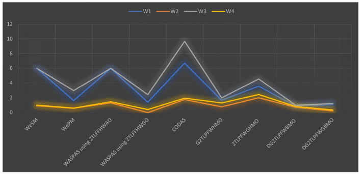
We have solved a problem of SWDLS for manufacturing plants in Manchester. For this purpose, we have used the extended 2TLFF-WASPAS method with Hamacher aggregation operators. We have solved the SWDLS problem by using the WASPAS method with the 2TLFFHWA operator and 2TLFFHWG operator. Also, we have solved the SWDLS problem using the extended-WeSM measure and extended-WePM measure. To check the feasibility of our proposed method, we have compared the SWDLS problem with the operators including G2TLPFWHMO [56], 2TLPFWGHMO, DG2TLPFWBMO [57] and DG2TLPFWGBMO. We have also compared it with the CODAS method [61] for 2TLPFNs. From the above analysis, we have the same best landfill location, i.e., $ W_3 $. The comparative analysis shows that the proposed WASPAS method yields valid results. Neither 2TLISs nor 2TLPFSs can handle the situation when the sum of squares of the 2-tuple linguistic MD and non-MD exceeds 1. Hence, it is necessary to develop a new model in this case. Also the proposed 2TLFF-WASPAS method is superior to the existing CODAS method [61], because the existing CODAS method [61] can only be used for 2TLPF data whereas the proposed method can be used for both 2TLPF data and 2TLFF data. The combined ranking of all above-mentioned applications is shown in Table 29. A graph of the ranking of all above-mentioned methods is shown in Figure 6.
| Methods | Ranking | Optimal Alternative |
| WASPAS method with 2TLFFHWA operator | $ W_3 > W_1 > W_4 > W_2 $ | $ W_3 $ |
| WASPAS method with 2TLFFHWG operator | $ W_3 > W_1 > W_4 > W_2 $ | $ W_3 $ |
| WeSM method with 2TLFFHWA operator | $ W_3= W_1 > W_4 > W_2 $ | $ W_3 $ and $ W_1 $ |
| WePM method with 2TLFFHWA operator | $ W_3 > W_1 > W_4 > W_2 $ | $ W_3 $ |
| CODAS method with 2TLPFNs [61] | $ W_3 > W_1 > W_4 > W_2 $ | $ W_3 $ |
| G2TLPFWHMO [56] | $ W_3 > W_1 > W_4 > W_2 $ | $ W_3 $ |
| 2TLPFWGHMO [56] | $ W_3 > W_1 > W_4 > W_2 $ | $ W_3 $ |
| DG2TLPFWBMO [57] | $ W_3 > W_1 > W_4 > W_2 $ | $ W_3 $ |
| DG2TLPFWGBMO [57] | $ W_3 > W_1 > W_4 > W_2 $ | $ W_3 $ |
DownLoad:
CSV
MAGDM methods have been widely used in the field of SWDLS problems. This study is the first to take into account the MAGDM of SWDLS in the context of 2TLFFSs. Many MAGDM techniques, though, which are used for evaluation with many criteria, have not yet been modified for this setting. One of the effective MAGDM techniques is the WASPAS approach, which has been used to solve numerous MAGDM issues in the real world. In this paper, a novel integrated strategy based on the WASPAS method is put forth to address MAGDM issues with 2TLFFNs. The principles and arithmetic operations of 2TFFSs have been applied in this technique to adapt the WASPAS method to 2TLFF information, and various modifications have been made in the process. In this work, we modified the WePM and WeSM processes, and we suggested an expanded WASPAS that can tackle MAGDM issues in such a scenario. Additionally, the SMART technique has been applied to get more accurate criteria weights using data with 2TLFFSs as a defining characteristic. One of the main issues with the decision-making process is the calculation of criteria weights. The proposed approach has been validated using a SWDLS example. To do this, the findings of the suggested strategy were compared to those of several other methods, and a sensitivity analysis was carried out by altering a method parameter. The analysis' findings indicate that the integrated strategy that has been suggested is valid for evaluating SWDLS and may work well for many other MAGDM issues.
1. The WASPAS method selects the option with the greatest utility, whereas previous methods prefer alternatives that are close to the ideal solution.
2. WASPAS is a combination of the WeSM and WePM and its accuracy is more consistent than the WePM and WeSM.
3. In the proposed 2TLFF-WASPAS, the standard weights are computed based on the SMART method [60], while in the CODAS method [61], Deng et al. [57] and Wei et al. [56], assuming standard weights, this leaves no room for dealing with ambiguity.
4. The advantages of the proposed WASPAS method include its efficiency of use in MCDM problems, the flexibility of using a FFS and 2-tuple LTs to define the information expressed by the DM and its applicability to various decision-making problems.
The WASPAS method is important among the available methods because of its ability to improve ranking accuracy. The 2TLFFS is a new generalization of the 2TLPFS and 2TLIFS, as it can handle more general cases than the 2TLPFS and 2TLIFS. In this research study, we have selected the best sites for manufacturing industrial solid waste in Manchester to dispose of. We have solved the SWDLS problem using the WASPAS method of the 2TLFFHWA operator. Furthermore, we have solved it using the WASPAS method for the 2TLFFHWG operator, WePM measurement and WeSM measurements. We also conducted a comparative study with existing methods [61] and operators, namely the G2TLPFWHMO [56], 2TLPFWGHMO [56] and DG2TLPFWBMO [57] DG2TLPFWGBMO [57] to show the applicability of its integrity.
Various MAGDM applications in other industries, i.e., agriculture, healthcare, etc., can be handled using the proposed technique. Certain new methods, such as double normalization-based multiple aggregation, gained and lost dominance score, ORESE, and measurement of alternatives and ranking according to the compromise solution in the fuzzy context of FFS and the 2TLFF can be used for future development. These methods can be used to solve SWDLS problems in different regions. Furthermore, the proposed 2TLFF-WASPAS method could be coupled with some other subjective criteria weighting methods such as analytic hierarchy process, Best Worst Method and analytic network process. Finally, the proposed method can be used to solve other emerging MAGDM problems.
The proposed method is based on FFS theory, which is a generalization of the PFS and IFS theories. Therefore, there are currently no significant limitations in the application of the proposed approach. The only real limitation that is observed is the selection of attributes. Only five attributes were selected, although many other factors, such as groundwater depth, proximity to surface water, elevation, land slope, soil permeability, soil stability, flooding susceptibility, lithology and stratification, faults, land use type, nearby settlements and urbanization, proximity to cultural and protected sites, wind direction, roads, railroads, proximity to building materials, pipelines, powerlines and proximity to airports are considered while selecting a disposal site. These factors can be considered in future studies.
The research of Santos-García was funded by the Spanish project ProCode-UCM (PID2019-108528RB-C22) from the Ministerio de Ciencia e Innovación.
The authors declare no conflict of interest.
| [1] |
Mattson MP (2000) Apoptosis in neurodegenerative disorders. Nat Rev Mol Cell Biol 1: 120-129. doi: 10.1038/35040009

|
| [2] |
Bredesen DE, Rao RV, Mehlen P (2006) Cell death in the nervous system. Nature 443: 796-802. doi: 10.1038/nature05293
|
| [3] |
Qin L, Wu X, Block ML, et al. (2007) Systemic LPS causes chronic neuroinflammation and progressive neurodegeneration. Glia 55: 453-462. doi: 10.1002/glia.20467
|
| [4] |
Tilleux S, Hermans E (2007) Neuroinflammation and regulation of glial glutamate uptake in neurological disorders. J Neurosci Res 85: 2059-2070. doi: 10.1002/jnr.21325
|
| [5] |
Sheldon AL, Robinson MB (2007) The role of glutamate transporters in neurodegenerative diseases and potential opportunities for intervention. Neurochem Int 51: 333-355. doi: 10.1016/j.neuint.2007.03.012
|
| [6] | Kostic M, Zivkovic N, Stojanovic I (2013) Multiple sclerosis and glutamate excitotoxicity. Rev Neurosci 24: 71-88. |
| [7] |
Morimoto K, Murasugi T, Oda T (2002) Acute neuroinflammation exacerbates excitotoxicity in rat hippocampus in vivo. Exp Neurol 177: 95-104. doi: 10.1006/exnr.2002.7991
|
| [8] |
Zou JY, Crews FT (2005) TNF alpha potentiates glutamate neurotoxicity by inhibiting glutamate uptake in organotypic brain slice cultures: neuroprotection by NF kappa B inhibition. Brain Res 1034: 11-24. doi: 10.1016/j.brainres.2004.11.014
|
| [9] |
Scaffidi P, Misteli T, Bianchi ME (2002) Release of chromatin protein HMGB1 by necrotic cells triggers inflammation. Nature 418: 191-195. doi: 10.1038/nature00858
|
| [10] |
Bell CW, Jiang W, Reich CF, et al. (2006) The extracellular release of HMGB1 during apoptotic cell death. Am J Physiol Cell Physiol 291: C1318-1325. doi: 10.1152/ajpcell.00616.2005
|
| [11] |
Zou JY, Crews FT (2014) Release of neuronal HMGB1 by Ethanol through decreased HDAC activity activates brain neuroimmune signaling. PloS One 9: e87915. doi: 10.1371/journal.pone.0087915
|
| [12] |
Evankovich J, Cho SW, Zhang R, et al. (2010) High mobility group box 1 release from hepatocytes during ischemia and reperfusion injury is mediated by decreased histone deacetylase activity. J Biol Chem 285: 39888-39897. doi: 10.1074/jbc.M110.128348
|
| [13] |
Lotze MT, Tracey KJ (2005) High-mobility group box 1 protein (HMGB1): nuclear weapon in the immune arsenal. Nat Rev Immunol 5: 331-342. doi: 10.1038/nri1594
|
| [14] |
Andersson U, Tracey KJ (2011) HMGB1 is a therapeutic target for sterile inflammation and infection. Annu Rev Immunol 29: 139-162. doi: 10.1146/annurev-immunol-030409-101323
|
| [15] | Tang D, Billiar TR, Lotze MT (2012) A Janus tale of two active high mobility group box 1 (HMGB1) redox states. Mol Med 18: 1360-1362. |
| [16] |
Janko C, Filipovic M, Munoz LE, et al. (2014) Redox modulation of HMGB1-related signaling. Antioxid Redox Signal 20: 1075-1085. doi: 10.1089/ars.2013.5179
|
| [17] | Magna M, Pisetsky DS (2014) The role of HMGB1 in the pathogenesis of inflammatory and autoimmune diseases. Mol Med 20: 138-146. |
| [18] |
Faraco G, Fossati S, Bianchi ME, et al. (2007) High mobility group box 1 protein is released by neural cells upon different stresses and worsens ischemic neurodegeneration in vitro and in vivo. J Neurochem 103: 590-603. doi: 10.1111/j.1471-4159.2007.04788.x
|
| [19] |
Kim JB, Sig Choi J, Yu YM, et al. (2006) HMGB1, a novel cytokine-like mediator linking acute neuronal death and delayed neuroinflammation in the postischemic brain. J Neurosci 26: 6413-6421. doi: 10.1523/JNEUROSCI.3815-05.2006
|
| [20] |
Lo Coco D, Veglianese P, Allievi E, et al. (2007) Distribution and cellular localization of high mobility group box protein 1 (HMGB1) in the spinal cord of a transgenic mouse model of ALS. Neurosci Lett 412: 73-77. doi: 10.1016/j.neulet.2006.10.063
|
| [21] | Crews FT, Qin L, Sheedy D, et al. (2012) High Mobility Group Box 1/Toll-like Receptor Danger Signaling Increases Brain Neuroimmune Activation in Alcohol Dependence. Biol Psychiatry 73: 602-612. |
| [22] |
Maroso M, Balosso S, Ravizza T, et al. (2010) Toll-like receptor 4 and high-mobility group box-1 are involved in ictogenesis and can be targeted to reduce seizures. Nat Med 16: 413-419. doi: 10.1038/nm.2127
|
| [23] |
Kim SW, Jin Y, Shin JH, et al. (2012) Glycyrrhizic acid affords robust neuroprotection in the postischemic brain via anti-inflammatory effect by inhibiting HMGB1 phosphorylation and secretion. Neurobiol Dis 46: 147-156. doi: 10.1016/j.nbd.2011.12.056
|
| [24] |
Ohnishi M, Katsuki H, Fukutomi C, et al. (2011) HMGB1 inhibitor glycyrrhizin attenuates intracerebral hemorrhage-induced injury in rats. Neuropharmacology 61: 975-980. doi: 10.1016/j.neuropharm.2011.06.026
|
| [25] |
Okuma Y, Liu K, Wake H, et al. (2014) Glycyrrhizin inhibits traumatic brain injury by reducing HMGB1-RAGE interaction. Neuropharmacology 85: 18-26. doi: 10.1016/j.neuropharm.2014.05.007
|
| [26] | Chavan SS, Huerta PT, Robbiati S, et al. (2012) HMGB1 mediates cognitive impairment in sepsis survivors. Molecular medicine 18: 930-937. |
| [27] |
Brana C, Benham C, Sundstrom L (2002) A method for characterising cell death in vitro by combining propidium iodide staining with immunohistochemistry. Brain Res Brain Res Protoc 10: 109-114. doi: 10.1016/S1385-299X(02)00201-5
|
| [28] |
Noraberg J, Kristensen BW, Zimmer J (1999) Markers for neuronal degeneration in organotypic slice cultures. Brain Res Brain Res Protoc 3: 278-290. doi: 10.1016/S1385-299X(98)00050-6
|
| [29] |
Zimmer J, Kristensen BW, Jakobsen B, et al. (2000) Excitatory amino acid neurotoxicity and modulation of glutamate receptor expression in organotypic brain slice cultures. Amino Acids 19: 7-21. doi: 10.1007/s007260070029
|
| [30] |
Koh JY, Choi DW (1987) Quantitative determination of glutamate mediated cortical neuronal injury in cell culture by lactate dehydrogenase efflux assay. J Neurosci Methods 20: 83-90. doi: 10.1016/0165-0270(87)90041-0
|
| [31] |
Zou JY, Crews FT (2005) TNF alpha potentiates glutamate neurotoxicity by inhibiting glutamate uptake in organotypic brain slice cultures: neuroprotection by NF kappa B inhibition. Brain Res 1034: 11-24. doi: 10.1016/j.brainres.2004.11.014
|
| [32] |
Balosso S, Liu J, Bianchi ME, et al. (2014) Disulfide-Containing High Mobility Group Box-1 Promotes N-Methyl-d-Aspartate Receptor Function and Excitotoxicity by Activating Toll-Like Receptor 4-Dependent Signaling in Hippocampal Neurons. Antioxid Redox Signal 21: 1726-1740. doi: 10.1089/ars.2013.5349
|
| [33] | Chenard BL, Menniti FS (1999) Antagonists selective for NMDA receptors containing the NR2B subunit. Curr Pharma Des 5: 381-404. |
| [34] |
Kim SW, Lim CM, Kim JB, et al. (2011) Extracellular HMGB1 released by NMDA treatment confers neuronal apoptosis via RAGE-p38 MAPK/ERK signaling pathway. Neurotox Res 20: 159-169. doi: 10.1007/s12640-010-9231-x
|
| [35] |
Glass CK, Saijo K, Winner B, et al. (2010) Mechanisms underlying inflammation in neurodegeneration. Cell 140: 918-934. doi: 10.1016/j.cell.2010.02.016
|
| [36] |
Crews FT, Qin L, Sheedy D, et al. (2013) High mobility group box 1/Toll-like receptor danger signaling increases brain neuroimmune activation in alcohol dependence. Biol Psychiatry 73: 602-612. doi: 10.1016/j.biopsych.2012.09.030
|
| [37] |
Kim JB, Lim CM, Yu YM, et al. (2008) Induction and subcellular localization of high-mobility group box-1 (HMGB1) in the postischemic rat brain. J Neurosci Res 86: 1125-1131. doi: 10.1002/jnr.21555
|
| [38] |
Qiu J, Nishimura M, Wang Y, et al. (2008) Early release of HMGB-1 from neurons after the onset of brain ischemia. J Cereb Blood Flow Metab 28: 927-938. doi: 10.1038/sj.jcbfm.9600582
|
| [39] | Choi DW (1987) Ionic dependence of glutamate neurotoxicity. J Neurosci 7: 369-379. |
| [40] |
Kim ID, Shin JH, Lee HK, et al. (2012) Intranasal delivery of HMGB1-binding heptamer peptide confers a robust neuroprotection in the postischemic brain. Neurosci Lett 525: 179-183. doi: 10.1016/j.neulet.2012.07.040
|
| [41] |
Sun Q, Wang F, Li W, et al. (2013) Glycyrrhizic acid confers neuroprotection after subarachnoid hemorrhage via inhibition of high mobility group box-1 protein: a hypothesis for novel therapy of subarachnoid hemorrhage. Med Hypotheses 81: 681-685. doi: 10.1016/j.mehy.2013.07.026
|
| [42] |
Zhang J, Wu Y, Weng Z, et al. (2014) Glycyrrhizin protects brain against ischemia-reperfusion injury in mice through HMGB1-TLR4-IL-17A signaling pathway. Brain Res 1582: 176-186. doi: 10.1016/j.brainres.2014.07.002
|
| [43] | Yang QW, Xiang J, Zhou Y, et al. (2010) Targeting HMGB1/TLR4 signaling as a novel approach to treatment of cerebral ischemia. Front Biosci 2: 1081-1091. |
| [44] |
Laird MD, Shields JS, Sukumari-Ramesh S, et al. (2014) High mobility group box protein-1 promotes cerebral edema after traumatic brain injury via activation of toll-like receptor 4. Glia 62: 26-38. doi: 10.1002/glia.22581
|
| [45] |
Maroso M, Balosso S, Ravizza T, et al. (2010) Toll-like receptor 4 and high-mobility group box-1 are involved in ictogenesis and can be targeted to reduce seizures. Nat Med 16: 413-419. doi: 10.1038/nm.2127
|
| 1. | Ibrahim M. Hezam, Pratibha Rani, Arunodaya Raj Mishra, Ahmad Alshamrani, An intuitionistic fuzzy entropy-based gained and lost dominance score decision-making method to select and assess sustainable supplier selection, 2023, 8, 2473-6988, 12009, 10.3934/math.2023606 | |
| 2. | Musavarah Sarwar, Improved assessment model for health-care waste management based on dual 2-tuple linguistic rough number clouds, 2023, 123, 09521976, 106255, 10.1016/j.engappai.2023.106255 | |
| 3. | Sumera Naz, Muhammad Ramzan Saeed, Shariq Aziz Butt, Multi-attribute group decision-making based on 2-tuple linguistic cubic q-rung orthopair fuzzy DEMATEL analysis, 2024, 9, 2364-4966, 10.1007/s41066-023-00433-7 | |
| 4. | Muhammad Akram, Sundas Shahzadi, Rabia Bibi, Gustavo Santos-García, Extended group decision-making methods with 2-tuple linguistic Fermatean fuzzy sets, 2023, 1432-7643, 10.1007/s00500-023-08158-0 | |
| 5. | Yuqi Zang, Jiamei Zhao, Wenchao Jiang, Tong Zhao, Advanced Linguistic Complex T-Spherical Fuzzy Dombi-Weighted Power-Partitioned Heronian Mean Operator and Its Application for Emergency Information Quality Assessment, 2024, 16, 2071-1050, 3069, 10.3390/su16073069 | |
| 6. | Mouhamed Bayane Bouraima, Yanjun Qiu, Ertugrul Ayyildiz, Aslihan Yildiz, Prioritization of strategies for a sustainable regional transportation infrastructure by hybrid spherical fuzzy group decision-making approach, 2023, 35, 0941-0643, 17967, 10.1007/s00521-023-08660-4 | |
| 7. | Muhammad Akram, Sundas Shahzadi, Syed Muhammad Umer Shah, Tofigh Allahviranloo, A fully Fermatean fuzzy multi-objective transportation model using an extended DEA technique, 2023, 8, 2364-4966, 1173, 10.1007/s41066-023-00399-6 | |
| 8. | Muhammad Akram, Arooj Adeel, 2023, Chapter 9, 978-3-031-43635-2, 437, 10.1007/978-3-031-43636-9_9 | |
| 9. | Abrar Hussain, Xiaoya Zhu, Kifayat Ullah, Dragan Pamucar, Muhammad Rashid, Shi Yin, Recycling of waste materials based on decision support system using picture fuzzy Dombi Bonferroni means, 2024, 1432-7643, 10.1007/s00500-023-09328-w | |
| 10. | Ertugrul Ayyildiz, Melike Erdogan, Literature analysis of the location selection studies related to the waste facilities within MCDM approaches, 2024, 1614-7499, 10.1007/s11356-024-34370-y | |
| 11. | Sumera Naz, Aqsa Shafiq, Shariq Aziz Butt, CILOS-WASPAS approach based on Schweizer–Sklar power operators for evaluating cosmetic brands in a group decision-making environment, 2024, 9, 2364-4966, 10.1007/s41066-024-00481-7 | |
| 12. | Rajkumar Verma, Eduardo Álvarez-Miranda, Multiple-attribute group decision-making approach using power aggregation operators with CRITIC-WASPAS method under 2-dimensional linguistic intuitionistic fuzzy framework, 2024, 157, 15684946, 111466, 10.1016/j.asoc.2024.111466 | |
| 13. | Sumera Naz, Aqsa Shafiq, Shariq Aziz Butt, Shahzra Mazhar, Diaz Jorge Martinez, Emiro De la Hoz Franco, Decision analysis with IDOCRIW-QUALIFLEX approach in the 2TLq-ROF environment: An application of accident prediction models in Pakistan, 2024, 10, 24058440, e27669, 10.1016/j.heliyon.2024.e27669 | |
| 14. | Palvinder Thakur, Neeraj Gandotra, Namita Saini, 2024, 3232, 0094-243X, 070004, 10.1063/5.0227865 | |
| 15. | Sumera Naz, Muhammad Akram, Muhammad Muneeb ul Hassan, Areej Fatima, A Hybrid DEMATEL-TOPSIS Approach Using 2-Tuple Linguistic q-Rung Orthopair Fuzzy Information and Its Application in Renewable Energy Resource Selection, 2024, 23, 0219-6220, 1099, 10.1142/S0219622023500323 | |
| 16. | Sumera Naz, Aqsa Shafiq, Shariq Aziz Butt, Rabia Tasneem, Dragan Pamucar, Zhoe Comas Gonzalez, Decision-making model for selecting products through online product reviews utilizing natural language processing techniques, 2025, 611, 09252312, 128593, 10.1016/j.neucom.2024.128593 | |
| 17. | Muhammad Akram, Safeena Azam, Mohammed M. Ali Al-Shamiri, Dragan Pamucar, An outranking method for selecting the best gate security system using spherical fuzzy rough numbers, 2024, 138, 09521976, 109411, 10.1016/j.engappai.2024.109411 | |
| 18. | Junbo Li, Fangwei Zhang, Rui Wang, Huan Ni, Taiyang Li, A comprehensive evaluation model for university classroom teaching quality based on machine vision and Fermatean fuzzy sets, 2023, 1432-7643, 10.1007/s00500-023-09426-9 | |
| 19. | S. P. Sundar Singh Sivam, N. Harshavardhana, D. Kumaran, Multi-criteria optimization model integrating fermatean fuzzy sets and WASPAS for enhancing copper strip quality in cold rolling, 2025, 8, 2520-8160, 10.1007/s41939-025-00784-5 | |
| 20. | Mustafa Güler, Yeşim Altay, 2025, Chapter 27, 978-3-031-83610-7, 371, 10.1007/978-3-031-83611-4_27 | |
| 21. | 国柔 万, WASPAS Multi-Attribute Decision-Making Method Based on Interval Valued Pythagorean Sugeno-Weber Softmax Operator, 2025, 14, 2324-7991, 174, 10.12677/aam.2025.147355 | |
| 22. | 国柔 万, Multi-Attribute Decision-Making Method Based on Neutrosophic Z-Number WASPAS, 2025, 14, 2324-7991, 134, 10.12677/aam.2025.147352 | |
| 23. | Abrar Hussain, Kifayat Ullah, Zeeshan Ali, Sarbast Moslem, Tapan Senapati, An Enhanced Physical Education Evaluation Algorithm for Higher Education Using Interval Valued Fermatean Fuzzy Information, 2025, 00380121, 102280, 10.1016/j.seps.2025.102280 |
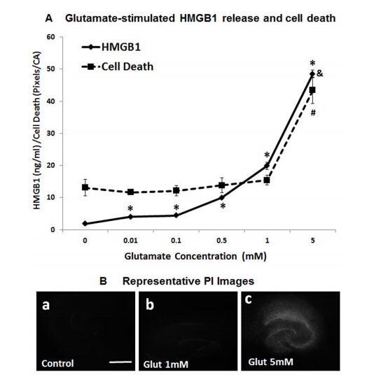
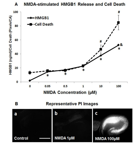
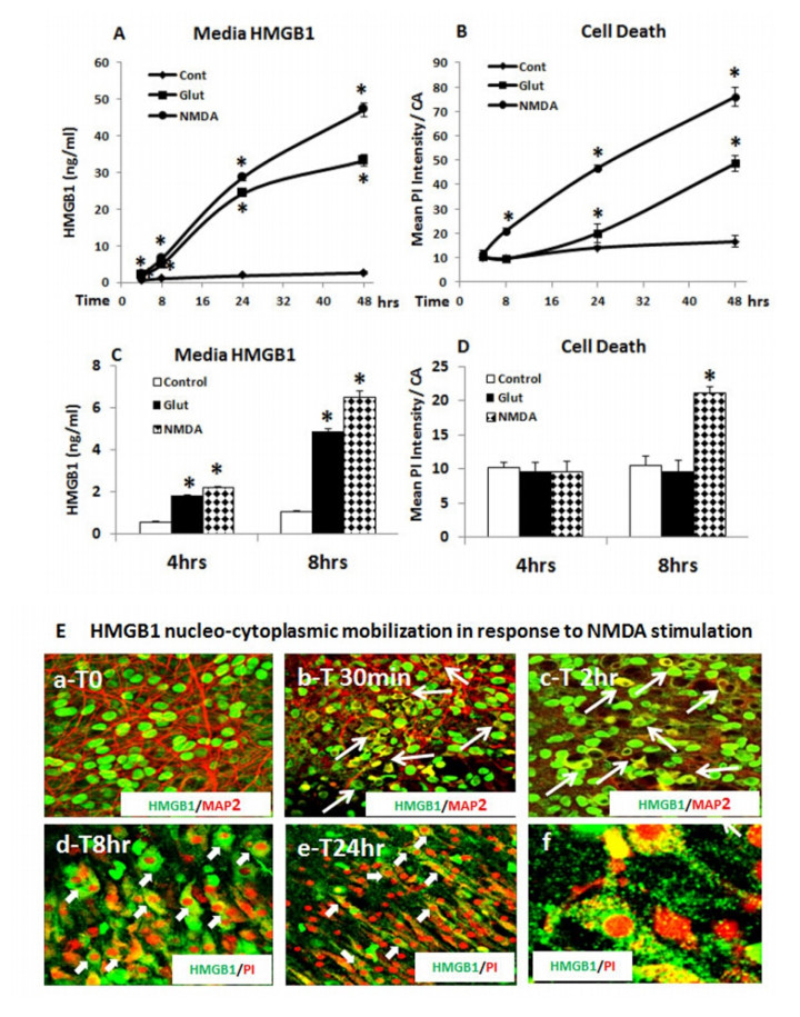
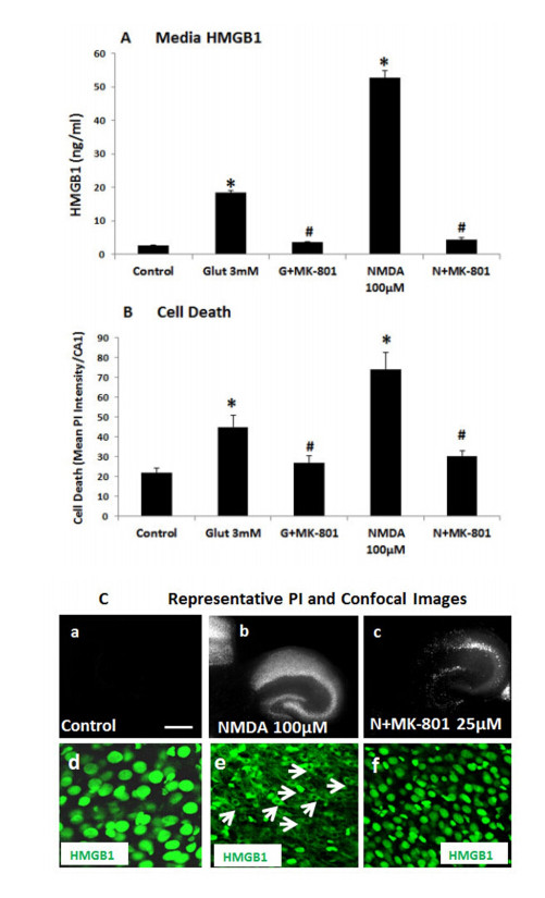
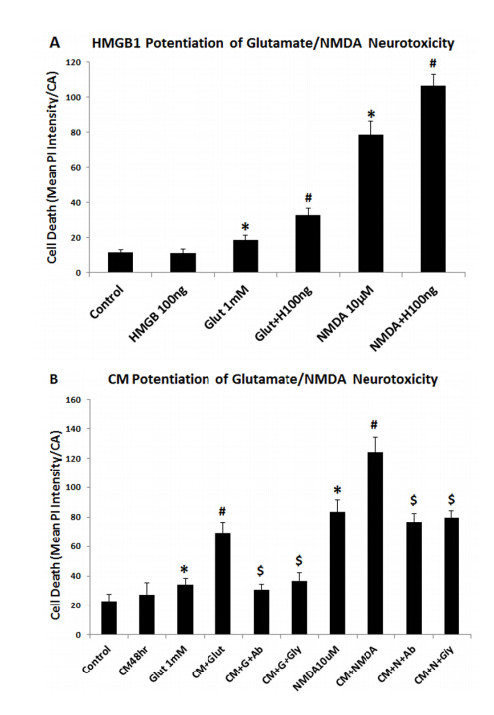
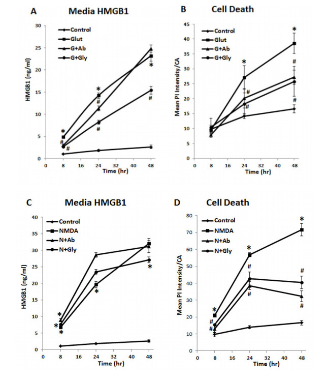
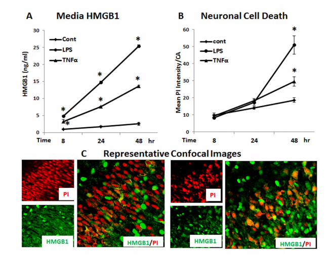
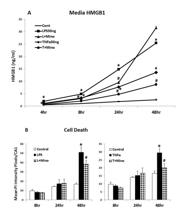
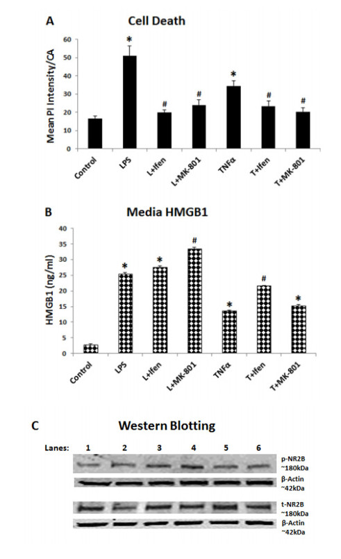
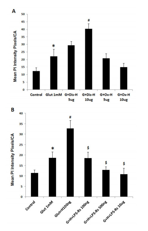
Figures(10)

Jian Zou, Fulton T. Crews. Glutamate/NMDA excitotoxicity and HMGB1/TLR4 neuroimmune toxicity converge as components of neurodegeneration[J]. AIMS Molecular Science, 2015, 2(2): 77-100. doi: 10.3934/molsci.2015.2.77

| Authors | Year | Significance influence |
| Zavadskas et al. [21] | 2012 | Proposed optimization of WASPAS |
| Antucheviciene et al. [28] | 2013 | Introduced MCDM methods WASPAS and MULTIMOORA |
| Lashgari et al. [29] | 2014 | Determined outsourcing strategies using QSPM and WASPAS methods |
| Zavadskas et al. [30] | 2014 | Designed WASPAS with interval-valued IF numbers |
| Chakraborty and Saparauskas [31] | 2014 | Proposed WASPAS method in manufacturing decision making |
| Chakraborty et al.[32] | 2015 | Studied WASPAS method as a MCDM tool |
| Zavadskas et al. [22] | 2015 | Presented the single-valued neurotrophic WASPAS |
| Zavadskas et al. [33] | 2015 | Studied WASPAS method as an optimization tool |
| Karabasevic et al. [34] | 2016 | Proposed a personnel selection method based on SWARA and WASPAS |
| Zavadskas et al. [35] | 2016 | Presented a multi-attribute assessment using WASPAS |
| Mardani et al. [36] | 2017 | Described a systematic review of SWARA and WASPAS |
| Mardani et al. [25] | 2017 | Introduced HF-SWOT-SWARA-WASPAS |
| Bausys and Juodagalvien [37] | 2017 | Investigated garage location selection using WASPAS-SVNS method |
| Stanujki and Karabasevi [38] | 2018 | Designed extension of the WASPAS method with IF numbers |
| Turskis et al. [39] | 2019 | Presented an F-WASPAS-based approach |
| Mishra et al. [23] | 2019 | Proposed the HF WASPAS |
| Schitea et al. [24] | 2019 | Described IF-WASPAS-COPRAS-EDAS |
| Gundogdu and Kahraman [40] | 2019 | Introduced WASPAS with spherical fuzzy sets |
| Dehshiri and Aghaei [41] | 2019 | Examined fuzzy Delphi, SWARA and WASPAS |
| Rani and Mishra [42] | 2020 | Proposed q-rung orthopair WASPAS |
| Mohagheghi and Mousavi [43] | 2020 | Introduced IVPF D-WASPAS |
| Rani et al. [27] | 2020 | Presented IF type-2 WASPAS |
| Sergi and Ucal Sari [44] | 2021 | Examined digitalization using fuzzy Z-WASPAS and fuzzy Z-AHP |
| Rudnik et al. [45] | 2021 | Introduced the ordered fuzzy WASPAS method |
| Badalpur and Nurbakhsh [46] | 2021 | Presented the WASPAS method for risk qualitative analysis |
| Pamucar et al. [47] | 2022 | Designed fuzzy Hamacher WASPAS decision-making model |
| This study | 2022 | Proposes 2-tuple linguistic Fermatean fuzzy WASPAS |
DownLoad:
CSV
| Alternatives | Site name |
| Astley sand and aggregated limited ($ W_1 $) | Morleys quarry |
| Augean north limited ($ W_2 $) | Marks Quarry Landfill site |
| Augean west limited ($ W_3 $) | Port Clarence non-hazardous landfill site |
| Augean south limited ($ W_4 $) | East Northants resource management facility |
DownLoad:
CSV
| Attribute | Type | Definition |
| Distance ($ T_1 $) | benefit | Distance from populated areas |
| Disease vector ($ T_2 $) | cost | Breeding of vectors in (e.g., rats, mosquitos) in landfill |
| Cost ($ T_3 $) | Cost | Land price, transportation cost and employee salary |
| Future development ($ T_4 $) | Benefit | possibility of development of land in future |
| Geographical circumstances ($ T_5 $) | Benefit | study of natural features of Earth's surface |
DownLoad:
CSV
| Attribute | Type | $ E_1 $ | $ E_2 $ | $ E_3 $ | Sum | $ w_j $ |
| Distance ($ T_1 $) | benefit | 80 | 70 | 85 | 235 | 0.23 |
| Disease vector ($ T_2 $) | cost | 40 | 30 | 60 | 130 | 0.13 |
| Cost ($ T_3 $) | cost | 90 | 90 | 80 | 260 | 0.26 |
| Future development ($ T_4 $) | benefit | 70 | 60 | 50 | 180 | 0.18 |
| Geographical circumstances ($ T_5 $) | benefit | 65 | 50 | 85 | 200 | 0.20 |
DownLoad:
CSV
| LV | 2TLFFNs |
| Very low ($ \ddot{VL} $) | $ \{(\bar{s}_0, 0), (\bar{s}_6, 0)\} $ |
| Low ($ \ddot{L} $) | $ \{(\bar{s}_1, 0), (\bar{s}_5, 0)\} $ |
| Medium Low ($ \ddot{ML} $) | $ \{(\bar{s}_2, 0), (\bar{s}_4, 0)\} $ |
| Medium ($ \ddot{M} $) | $ \{(\bar{s}_3, 0), (\bar{s}_3, 0)\} $ |
| Medium High ($ \ddot{MH} $) | $ \{(\bar{s}_4, 0), (\bar{s}_2, 0)\} $ |
| High ($ \ddot{H} $) | $ \{(\bar{s}_5, 0), (\bar{s}_1, 0)\} $ |
| Very High ($ \ddot{VH} $) | $ \{(\bar{s}_6, 0), (\bar{s}_0, 0)\} $ |
DownLoad:
CSV
| DMs | Sites | $ T_1 $ | $ T_2 $ | $ T_3 $ | $ T_4 $ | $ T_5 $ |
| $ E_1 $ | $ W_1 $ | $ \ddot{H} $ | $ \ddot{H} $ | $ \ddot{L} $ | $ \ddot{L} $ | $ \ddot{MH} $ |
| $ W_2 $ | $ \ddot{M} $ | $ \ddot{ML} $ | $ \ddot{MH} $ | $ \ddot{L} $ | $ \ddot{ML} $ | |
| $ W_3 $ | $ \ddot{L} $ | $ \ddot{H} $ | $ \ddot{H} $ | $ \ddot{M} $ | $ \ddot{VH} $ | |
| $ W_4 $ | $ \ddot{L} $ | $ \ddot{MH} $ | $ \ddot{M} $ | $ \ddot{H} $ | $ \ddot{L} $ | |
| $ E_2 $ | $ W_1 $ | $ \ddot{H} $ | $ \ddot{H} $ | $ \ddot{L} $ | $ \ddot{M} $ | $ \ddot{M} $ |
| $ W_2 $ | $ \ddot{M} $ | $ \ddot{M} $ | $ \ddot{MH} $ | $ \ddot{H} $ | $ \ddot{H} $ | |
| $ W_3 $ | $ \ddot{VH} $ | $ \ddot{H} $ | $ \ddot{MH} $ | $ \ddot{M} $ | $ \ddot{VH} $ | |
| $ W_4 $ | $ \ddot{L} $ | $ \ddot{L} $ | $ \ddot{M} $ | $ \ddot{MH} $ | $ \ddot{L} $ | |
| $ E_3 $ | $ W_1 $ | $ \ddot{H} $ | $ \ddot{VH} $ | $ \ddot{H} $ | $ \ddot{MH} $ | $ \ddot{MH} $ |
| $ W_2 $ | $ \ddot{M} $ | $ \ddot{L} $ | $ \ddot{L} $ | $ \ddot{L} $ | $ \ddot{ML} $ | |
| $ W_3 $ | $ \ddot{H} $ | $ \ddot{H} $ | $ \ddot{H} $ | $ \ddot{M} $ | $ \ddot{MH} $ | |
| $ W_4 $ | $ \ddot{H} $ | $ \ddot{H} $ | $ \ddot{M} $ | $ \ddot{H} $ | $ \ddot{H} $ |
DownLoad:
CSV
| DMs | Sites | $ T_1 $ | $ T_2 $ | $ T_3 $ | $ T_4 $ | $ T_5 $ |
| $ E_1 $ | $ W_1 $ | $ \{(\bar{s}_5, 0), (\bar{s}_1, 0)\} $ | $ \{(\bar{s}_5, 0), (\bar{s}_1, 0)\} $ | $ \{(\bar{s}_1, 0), (\bar{s}_5, 0)\} $ | $ \{(\bar{s}_1, 0), (\bar{s}_5, 0)\} $ | $ \{(\bar{s}_4, 0), (\bar{s}_2, 0)\} $ |
| $ W_2 $ | $ \{(\bar{s}_3, 0), (\bar{s}_3, 0)\} $ | $ \{(\bar{s}_2, 0), (\bar{s}_4, 0)\} $ | $ \{(\bar{s}_1, 0), (\bar{s}_5, 0)\} $ | $ \{(\bar{s}_1, 0), (\bar{s}_5, 0)\} $ | $ \{(\bar{s}_2, 0), (\bar{s}_4, 0)\} $ | |
| $ W_3 $ | $ \{(\bar{s}_1, 0), (\bar{s}_5, 0)\} $ | $ \{(\bar{s}_5, 0), (\bar{s}_1, 0)\} $ | $ \{(\bar{s}_5, 0), (\bar{s}_1, 0)\} $ | $ \{(\bar{s}_3, 0), (\bar{s}_3, 0)\} $ | $ \{(\bar{s}_6, 0), (\bar{s}_0, 0)\} $ | |
| $ W_4 $ | $ \{(\bar{s}_1, 0), (\bar{s}_5, 0)\} $ | $ \{(\bar{s}_4, 0), (\bar{s}_2, 0)\} $ | $ \{(\bar{s}_3, 0), (\bar{s}_3, 0)\} $ | $ \{(\bar{s}_5, 0), (\bar{s}_1, 0)\} $ | $ \{(\bar{s}_1, 0), (\bar{s}_5, 0)\} $ | |
| $ E_2 $ | $ W_1 $ | $ \{(\bar{s}_5, 0), (\bar{s}_1, 0)\} $ | $ \{(\bar{s}_5, 0), (\bar{s}_1, 0)\} $ | $ \{(\bar{s}_1, 0), (\bar{s}_5, 0)\} $ | $ \{(\bar{s}_3, 0), (\bar{s}_3, 0)\} $ | $ \{(\bar{s}_3, 0), (\bar{s}_3, 0)\} $ |
| $ W_2 $ | $ \{(\bar{s}_3, 0), (\bar{s}_3, 0)\} $ | $ \{(\bar{s}_3, 0), (\bar{s}_3, 0)\} $ | $ \{(\bar{s}_4, 0), (\bar{s}_2, 0)\} $ | $ \{(\bar{s}_5, 0), (\bar{s}_1, 0)\} $ | $ \{(\bar{s}_5, 0), (\bar{s}_1, 0)\} $ | |
| $ W_3 $ | $ \{(\bar{s}_6, 0), (\bar{s}_0, 0)\} $ | $ \{(\bar{s}_5, 0), (\bar{s}_1, 0)\} $ | $ \{(\bar{s}_4, 0), (\bar{s}_2, 0)\} $ | $ \{(\bar{s}_3, 0), (\bar{s}_3, 0)\} $ | $ \{(\bar{s}_6, 0), (\bar{s}_0, 0)\} $ | |
| $ W_4 $ | $ \{(\bar{s}_1, 0), (\bar{s}_5, 0)\} $ | $ \{(\bar{s}_1, 0), (\bar{s}_5, 0)\} $ | $ \{(\bar{s}_3, 0), (\bar{s}_3, 0)\} $ | $ \{(\bar{s}_4, 0), (\bar{s}_2, 0)\} $ | $ \{(\bar{s}_0, 0), (\bar{s}_6, 0)\} $ | |
| $ E_3 $ | $ W_1 $ | $ \{(\bar{s}_5, 0), (\bar{s}_1, 0)\} $ | $ \{(\bar{s}_6, 0), (\bar{s}_0, 0)\} $ | $ \{(\bar{s}_5, 0), (\bar{s}_1, 0)\} $ | $ \{(\bar{s}_4, 0), (\bar{s}_2, 0)\} $ | $ \{(\bar{s}_4, 0), (\bar{s}_2, 0)\} $ |
| $ W_2 $ | $ \{(\bar{s}_3, 0), (\bar{s}_3, 0)\} $ | $ \{(\bar{s}_1, 0), (\bar{s}_5, 0)\} $ | $ \{(\bar{s}_1, 0), (\bar{s}_5, 0)\} $ | $ \{(\bar{s}_1, 0), (\bar{s}_5, 0)\} $ | $ \{(\bar{s}_2, 0), (\bar{s}_4, 0)\} $ | |
| $ W_3 $ | $ \{(\bar{s}_5, 0), (\bar{s}_1, 0)\} $ | $ \{(\bar{s}_5, 0), (\bar{s}_1, 0)\} $ | $ \{(\bar{s}_5, 0), (\bar{s}_1, 0)\} $ | $ \{(\bar{s}_3, 0), (\bar{s}_3, 0)\} $ | $ \{(\bar{s}_4, 0), (\bar{s}_2, 0)\} $ | |
| $ W_4 $ | $ \{(\bar{s}_5, 0), (\bar{s}_1, 0)\} $ | $ \{(\bar{s}_5, 0), (\bar{s}_1, 0)\} $ | $ \{(\bar{s}_3, 0), (\bar{s}_3, 0)\} $ | $ \{(\bar{s}_5, 0), (\bar{s}_1, 0)\} $ | $ \{(\bar{s}_5, 0), (\bar{s}_1, 0)\} $ |
DownLoad:
CSV
| Sites | $ T_1 $ | $ T_2 $ | $ T_3 $ | $ T_4 $ | $ T_5 $ |
| $ W_1 $ | $ \{(\bar{s}_5, 0), (\bar{s}_1, 0)\} $ | $ \{(\bar{s}_6, 0), (\bar{s}_0, 0)\} $ | $ \{(\bar{s}_4, -0.33), (\bar{s}_3, 0.5)\} $ | $ \{(\bar{s}_3, 0.25), (\bar{s}_3, -0.05)\} $ | $ \{(\bar{s}_4, -0.40), (\bar{s}_2, 0.44)\} $ |
| $ W_2 $ | $ \{(\bar{s}_3, 0), (\bar{s}_3, 0)\} $ | $ \{(\bar{s}_2, 0.5), (\bar{s}_4, -0.29)\} $ | $ \{(\bar{s}_4, -0.38), (\bar{s}_3, -0.63)\} $ | $ \{(\bar{s}_4, 0.23), (\bar{s}_2, 0.44)\} $ | $ \{(\bar{s}_4, 0.28), (\bar{s}_2, 0)\} $ |
| $ W_3 $ | $ \{(\bar{s}_6, 0), (\bar{s}_0, 0)\} $ | $ \{(\bar{s}_5, 0), (\bar{s}_1, 0)\} $ | $ \{(\bar{s}_5, -0.38), (\bar{s}_1, 0.41)\} $ | $ \{(\bar{s}_3, 0), (\bar{s}_3, 0)\} $ | $ \{(\bar{s}_6, 0), (\bar{s}_0, 0)\} $ |
| $ W_4 $ | $ \{(\bar{s}_4, -0.33), (\bar{s}_3, 0.50)\} $ | $ \{(\bar{s}_4, -0.06), (\bar{s}_3, -0.43)\} $ | $ \{(\bar{s}_3, 0), (\bar{s}_3, 0)\} $ | $ \{(\bar{s}_5, -0.38), (\bar{s}_1, 0.41)\} $ | $ \{(\bar{s}_4, -0.32), (\bar{s}_3, 0.37)\} $ |
DownLoad:
CSV
| Sites | $ T_1 $ | $ T_2 $ | $ T_3 $ | $ T_4 $ | $ T_5 $ |
| $ W_1 $ | $ \{(\bar{s}_6, 0), (\bar{s}_0, 0)\} $ | $ \{(\bar{s}_0, 0), (\bar{s}_6, 0)\} $ | $ \{(\bar{s}_3, 0.5), (\bar{s}_4, -0.33)\} $ | $ \{(\bar{s}_3, 0.25), (\bar{s}_3, -0.05)\} $ | $ \{(\bar{s}_4, -0.40), (\bar{s}_2, 0.44)\} $ |
| $ W_2 $ | $ \{(\bar{s}_3, 0), (\bar{s}_3, 0)\} $ | $ \{(\bar{s}_4, -0.29), (\bar{s}_2, 0.5)\} $ | $ \{(\bar{s}_3, -0.63), (\bar{s}_4, -0.38)\} $ | $ \{(\bar{s}_4, 0.23), (\bar{s}_2, 0.44)\} $ | $ \{(\bar{s}_4, 0.28), (\bar{s}_2, 0)\} $ |
| $ W_3 $ | $ \{(\bar{s}_6, 0), (\bar{s}_0, 0)\} $ | $ \{(\bar{s}_1, 0), (\bar{s}_5, 0) \} $ | $ \{(\bar{s}_1, 0.41), (\bar{s}_5, -0.38)\} $ | $ \{(\bar{s}_3, 0), (\bar{s}_3, 0)\} $ | $ \{(\bar{s}_6, 0), (\bar{s}_0, 0)\} $ |
| $ W_4 $ | $ \{(\bar{s}_4, -0.33), (\bar{s}_3, 0.50)\} $ | $ \{(\bar{s}_3, -0.43), (\bar{s}_4, -0.06)\} $ | $ \{(\bar{s}_3, 0), (\bar{s}_3, 0)\} $ | $ \{(\bar{s}_5, -0.38), (\bar{s}_1, 0.41)\} $ | $ \{(\bar{s}_4, -0.32), (\bar{s}_3, 0.37)\} $ |
DownLoad:
CSV
| Sites | $ L_{ij}^{s} $ | $ L_{ij}^p $ | $ L_{ij} $ |
| $ W_1 $ | $ \{(\bar{s}_6, 0), (\bar{s}_0, 0)\} $ | $ \{(\bar{s}_4, 0.26), (\bar{s}_3, -0.30)\} $ | $ \{(\bar{s}_6, 0), (\bar{s}_0, 0.01)\} $ |
| $ W_2 $ | $ \{(\bar{s}_4, -0.28), (\bar{s}_3, -0.35)\} $ | $ \{(\bar{s}_4, -0.48), (\bar{s}_3, -0.18)\} $ | $ \{(\bar{s}_4, -0.37), (\bar{s}_0, 0.01)\} $ |
| $ W_3 $ | $ \{(\bar{s}_6, 0), (\bar{s}_0, 0)\} $ | $ \{(\bar{s}_5, -0.16), (\bar{s}_2, -0.18)\} $ | $ \{(\bar{s}_6, 0), (\bar{s}_0, 0)\} $ |
| $ W_4 $ | $ \{(\bar{s}_4, -0.18), (\bar{s}_3, -0.32)\} $ | $ \{(\bar{s}_4, -0.33), (\bar{s}_3, 0.03)\} $ | $ \{(\bar{s}_3, -0.25), (\bar{s}_0, 0.05)\} $ |
DownLoad:
CSV
| Sites | $ \dot{S}(L_{ij}) $ | Ranking |
| $ W_1 $ | 5.999 | 2 |
| $ W_2 $ | 1.3208 | 4 |
| $ W_3 $ | 6 | 1 |
| $ W_4 $ | 1.45859 | 3 |
DownLoad:
CSV
| Sites | $ T_1 $ | $ T_2 $ | $ T_3 $ | $ T_4 $ | $ T_5 $ |
| $ W_1 $ | $ \{(\bar{s}_5, 0.47), (\bar{s}_1, -0.20)\} $ | $ \{(\bar{s}_5, 0.28), (\bar{s}_1, -0.11)\} $ | $ \{(\bar{s}_2, -0.38), (\bar{s}_5, -0.38)\} $ | $ \{(\bar{s}_3, -0.37), (\bar{s}_4, -0.36)\} $ | $ \{(\bar{s}_3, 0.46), (\bar{s}_3, -0.39)\} $ |
| $ W_2 $ | $ \{(\bar{s}_3, 0), (\bar{s}_3, 0)\} $ | $ \{(\bar{s}_2, -0.01), (\bar{s}_4, 0.13)\} $ | $ \{(\bar{s}_3, -0.36), (\bar{s}_4, -0.22)\} $ | $ \{(\bar{s}_2, 0.23), (\bar{s}_4, 0.23)\} $ | $ \{(\bar{s}_3, 0.16), (\bar{s}_3, 0.27)\} $ |
| $ W_3 $ | $ \{(\bar{s}_4, -0.04), (\bar{s}_3, 0.25)\} $ | $ \{(\bar{s}_5, 0), (\bar{s}_1, 0)\} $ | $ \{(\bar{s}_4, 0.47), (\bar{s}_2, -0.34)\} $ | $ \{(\bar{s}_3, 0), (\bar{s}_3, 0)\} $ | $ \{(\bar{s}_5, 0.31), (\bar{s}_1, 0.34)\} $ |
| $ W_4 $ | $ \{(\bar{s}_2, -0.38), (\bar{s}_5, -0.39)\} $ | $ \{(\bar{s}_2, 0.13), (\bar{s}_4, 0.25)\} $ | $ \{(\bar{s}_3, 0), (\bar{s}_3, 0)\} $ | $ \{(\bar{s}_4, 0.47), (\bar{s}_2, -0.34)\} $ | $ \{(\bar{s}_2, -0.38), (\bar{s}_5, -0.38)\} $ |
DownLoad:
CSV
| Sites | $ T_1 $ | $ T_2 $ | $ T_3 $ | $ T_4 $ | $ T_5 $ |
| $ W_1 $ | $ \{(\bar{s}_5, 0.47), (\bar{s}_1, -0.20)\} $ | $ \{ (\bar{s}_1, -0.11), (\bar{s}_5, 0.28)\} $ | $ \{(\bar{s}_5, -0.38), (\bar{s}_2, -0.38) \} $ | $ \{(\bar{s}_3, -0.37), (\bar{s}_4, -0.36)\} $ | $ \{(\bar{s}_3, 0.46), (\bar{s}_3, -0.39)\} $ |
| $ W_2 $ | $ \{(\bar{s}_3, 0), (\bar{s}_3, 0)\} $ | $ \{ (\bar{s}_4, 0.13), (\bar{s}_2, -0.01)\} $ | $ \{(\bar{s}_4, -0.22), (\bar{s}_3, -0.36) \} $ | $ \{(\bar{s}_2, 0.23), (\bar{s}_4, 0.23)\} $ | $ \{(\bar{s}_3, 0.16), (\bar{s}_3, 0.27)\} $ |
| $ W_3 $ | $ \{(\bar{s}_4, -0.04), (\bar{s}_3, 0.25)\} $ | $ \{ (\bar{s}_1, 0), (\bar{s}_5, 0)\} $ | $ \{ (\bar{s}_2, -0.34), (\bar{s}_4, 0.47)\} $ | $ \{(\bar{s}_3, 0), (\bar{s}_3, 0)\} $ | $ \{(\bar{s}_5, 0.31), (\bar{s}_1, 0.34)\} $ |
| $ W_4 $ | $ \{(\bar{s}_2, -0.38), (\bar{s}_5, -0.39)\} $ | $ \{ (\bar{s}_4, 0.25), (\bar{s}_2, 0.13)\} $ | $ \{(\bar{s}_3, 0), (\bar{s}_3, 0)\} $ | $ \{(\bar{s}_4, 0.47), (\bar{s}_2, -0.34)\} $ | $ \{(\bar{s}_2, -0.38), (\bar{s}_5, -0.39)\} $ |
DownLoad:
CSV
| Sites | $ L_{ij}^{s} $ | $ L_{ij}^p $ | $ L_{ij} $ |
| $ W_1 $ | $ \{(\bar{s}_4, -0.29), (\bar{s}_0, 0.28)\} $ | $ \{(\bar{s}_3, -0.45), (\bar{s}_0, 0.44)\} $ | $ \{(\bar{s}_4, -0.01), (\bar{s}_0, 0.021)\} $ |
| $ W_2 $ | $ \{(\bar{s}_2, 0.19), (\bar{s}_0, 0.40)\} $ | $ \{(\bar{s}_2, 0.1), (\bar{s}_0, 0.48)\} $ | $ \{(\bar{s}_3, -0.31), (\bar{s}_0, 0.03)\} $ |
| $ W_3 $ | $ \{(\bar{s}_4, -0.2), (\bar{s}_0, 0.106)\} $ | $ \{(\bar{s}_3.0.49), (\bar{s}_0, 0.26)\} $ | $ \{(\bar{s}_4, 0.43), (\bar{s}_0, 0.004)\} $ |
| $ W_4 $ | $ \{(\bar{s}_2, 0.47), (\bar{s}_1, 0)\} $ | $ \{(\bar{s}_2, -0.12), (\bar{s}_1, 0)\} $ | $ \{(\bar{s}_3, -0.22), (\bar{s}_0, 0.16)\} $ |
DownLoad:
CSV
| Sites | $ \dot{S}(L_{ij}) $ | Ranking |
| $ W_1 $ | 1.7757 | 2 |
| $ W_2 $ | 0.53986 | 4 |
| $ W_3 $ | 2.41718 | 1 |
| $ W_4 $ | 0.59495 | 3 |
DownLoad:
CSV
| Sites | $ L_{ij}^{s} $ | $ L_{ij}^p $ | $ L_{ij} $ |
| $ W_1 $ | $ \{(\bar{s}_6, 0), (\bar{s}_0, 0)\} $ | $ \{(\bar{s}_4, 0.26), (\bar{s}_3, -0.30)\} $ | $ \{(\bar{s}_6, 0), (\bar{s}_0, 0.01)\} $ |
| $ W_2 $ | $ \{(\bar{s}_4, -0.28), (\bar{s}_3, -0.35)\} $ | $ \{(\bar{s}_4, -0.48), (\bar{s}_3, -0.18)\} $ | $ \{(\bar{s}_4, -0.28), (\bar{s}_3, -0.35)\} $ |
| $ W_3 $ | $ \{(\bar{s}_6, 0), (\bar{s}_0, 0)\} $ | $ \{(\bar{s}_5, -0.16), (\bar{s}_2, -0.18)\} $ | $ \{(\bar{s}_6, 0), (\bar{s}_0, 0)\} $ |
| $ W_4 $ | $ \{(\bar{s}_4, -0.18), (\bar{s}_3, -0.32)\} $ | $ \{(\bar{s}_4, -0.33), (\bar{s}_3, 0.03)\} $ | $ \{(\bar{s}_4, -0.18), (\bar{s}_3, -0.32)\} $ |
DownLoad:
CSV
| Sites | $ \dot{S}(L_{ij}) $ | Ranking |
| $ W_1 $ | 6 | 1 |
| $ W_2 $ | 0.9161 | 3 |
| $ W_3 $ | 6 | 1 |
| $ W_4 $ | 0.9885 | 2 |
DownLoad:
CSV
| Sites | $ L_{ij}^{s} $ | $ L_{ij}^p $ | $ L_{ij} $ |
| $ W_1 $ | $ \{(\bar{s}_6, 0), (\bar{s}_0, 0)\} $ | $ \{(\bar{s}_4, 0.26), (\bar{s}_3, -0.30)\} $ | $ \{(\bar{s}_4, 0.26), (\bar{s}_3, -0.30)\} $ |
| $ W_2 $ | $ \{(\bar{s}_4, -0.28), (\bar{s}_3, -0.35)\} $ | $ \{(\bar{s}_4, -0.48), (\bar{s}_3, -0.18)\} $ | $ \{(\bar{s}_4, -0.48), (\bar{s}_3, -0.18)\} $ |
| $ W_3 $ | $ \{(\bar{s}_6, 0), (\bar{s}_0, 0)\} $ | $ \{(\bar{s}_5, -0.16), (\bar{s}_2, -0.18)\} $ | $ \{(\bar{s}_5, -0.16), (\bar{s}_2, -0.18)\} $ |
| $ W_4 $ | $ \{(\bar{s}_4, -0.18), (\bar{s}_3, -0.32)\} $ | $ \{(\bar{s}_5, -0.16), (\bar{s}_2, -0.18)\} $ | $ \{(\bar{s}_5, -0.16), (\bar{s}_2, -0.18)\} $ |
DownLoad:
CSV
| Sites | $ \dot{S}(L_{ij}) $ | Ranking |
| $ W_1 $ | 1.6181 | 2 |
| $ W_2 $ | 0.58762 | 4 |
| $ W_3 $ | 2.96668 | 1 |
| $ W_4 $ | 0.59008 | 3 |
DownLoad:
CSV
| Parameter | $ \dot{S}(W_1) $ | $ \dot{S}(W_2) $ | $ \dot{S}(W_3) $ | $ \dot{S}(W_4) $ | Ranking |
| $ \gamma=1 $ | $ (\bar{s}_6, -0.0001) $ | $ (\bar{s}_4, -0.29) $ | $ (\bar{s}_6, 0) $ | $ (\bar{s}_4, -0.34) $ | $ W_3 > W_1 > W_2 > W_4 $ |
| $ \gamma=2 $ | $ (\bar{s}_6, -0.00001) $ | $ (\bar{s}_4, -0.30) $ | $ (\bar{s}_6, 0) $ | $ (\bar{s}_3, 0.34) $ | $ W_3 > W_1 > W_2 > W_4 $ |
| $ \gamma=3 $ | $ (\bar{s}_6, -0.00001) $ | $ (\bar{s}_4, -0.31) $ | $ (\bar{s}_6, 0) $ | $ (\bar{s}_3, 0.41) $ | $ W_3 > W_1 > W_2 > W_4 $ |
| $ \gamma=4 $ | $ (\bar{s}_6, -0.000001) $ | $ (\bar{s}_3, 0.32) $ | $ (\bar{s}_6, 0) $ | $ (\bar{s}_3, 0.33) $ | $ W_3 > W_1 > W_2 > W_4 $ |
| $ \gamma=5 $ | $ (\bar{s}_6, -0.000001) $ | $ (\bar{s}_3, 0.33) $ | $ (\bar{s}_6, 0) $ | $ (\bar{s}_3, 0.33) $ | $ W_3 > W_1 > W_2 > W_4 $ |
| $ \gamma=6 $ | $ (\bar{s}_6, -0.000001) $ | $ (\bar{s}_3, 0.34) $ | $ (\bar{s}_6, 0) $ | $ (\bar{s}_3, 0.33) $ | $ W_3 > W_1 > W_2 > W_4 $ |
DownLoad:
CSV
| Parameter | $ \dot{S}(W_1) $ | $ \dot{S}(W_2) $ | $ \dot{S}(W_3) $ | $ \dot{S}(W_4) $ | Ranking |
| $ \gamma=1 $ | $ (\bar{s}_2, 0.25) $ | $ (\bar{s}_2, 0.12) $ | $ (\bar{s}_3, -0.08) $ | $ (\bar{s}_2, -0.13) $ | $ W_3 > W_1 > W_2 > W_4 $ |
| $ \gamma=2 $ | $ (\bar{s}_2, 0.32) $ | $ (\bar{s}_2, 0.15) $ | $ (\bar{s}_3, -0.17) $ | $ (\bar{s}_2, -0.06) $ | $ W_3 > W_1 > W_2 > W_4 $ |
| $ \gamma=3 $ | $ (\bar{s}_2, 0.37) $ | $ (\bar{s}_2, 0.17) $ | $ (\bar{s}_3, -0.19) $ | $ (\bar{s}_2, -0.04) $ | $ W_3 > W_1 > W_2 > W_4 $ |
| $ \gamma=4 $ | $ (\bar{s}_2, 0.40) $ | $ (\bar{s}_2, 0.18) $ | $ (\bar{s}_3, -0.19) $ | $ (\bar{s}_2, 0) $ | $ W_3 > W_1 > W_2 > W_4 $ |
| $ \gamma=5 $ | $ (\bar{s}_2, 0.43) $ | $ (\bar{s}_2, 0.19) $ | $ (\bar{s}_3, -0.19) $ | $ (\bar{s}_2, 0.03) $ | $ W_3 > W_1 > W_2 > W_4 $ |
| $ \gamma=6 $ | $ (\bar{s}_2, 0.45) $ | $ (\bar{s}_2, 0.19) $ | $ (\bar{s}_3, -0.19) $ | $ (\bar{s}_2, 0.05) $ | $ W_3 > W_1 > W_2 > W_4 $ |
DownLoad:
CSV
| Sites | $ T_1 $ | $ T_2 $ | $ T_3 $ | $ T_4 $ | $ T_5 $ |
| $ W_1 $ | $ \{(\bar{s}_6, 0), (\bar{s}_0, 0)\} $ | $ \{(\bar{s}_5, 0), (\bar{s}_1, 0)\} $ | $ \{(\bar{s}_1, 0), (\bar{s}_5, 0)\} $ | $ \{(\bar{s}_1, 0), (\bar{s}_5, 0)\} $ | $ \{(\bar{s}_4, 0), (\bar{s}_2, 0)\} $ |
| $ W_2 $ | $ \{(\bar{s}_3, 0), (\bar{s}_3, 0)\} $ | $ \{(\bar{s}_2, 0), (\bar{s}_4, 0)\} $ | $ \{(\bar{s}_1, 0), (\bar{s}_5, 0)\} $ | $ \{(\bar{s}_1, 0), (\bar{s}_5, 0)\} $ | $ \{(\bar{s}_2, 0), (\bar{s}_4, 0)\} $ |
| $ W_3 $ | $ \{(\bar{s}_1, 0), (\bar{s}_5, 0)\} $ | $ \{(\bar{s}_5, 0), (\bar{s}_1, 0)\} $ | $ \{(\bar{s}_5, 0), (\bar{s}_1, 0)\} $ | $ \{(\bar{s}_3, 0), (\bar{s}_3, 0)\} $ | $ \{(\bar{s}_6, 0), (\bar{s}_0, 0)\} $ |
| $ W_4 $ | $ \{(\bar{s}_1, 0), (\bar{s}_5, 0)\} $ | $ \{(\bar{s}_4, 0), (\bar{s}_2, 0)\} $ | $ \{(\bar{s}_3, 0), (\bar{s}_3, 0)\} $ | $ \{(\bar{s}_5, 0), (\bar{s}_1, 0)\} $ | $ \{(\bar{s}_1, 0), (\bar{s}_5, 0)\} $ |
DownLoad:
CSV
| Sites | $ T_1 $ | $ T_2 $ | $ T_3 $ | $ T_4 $ | $ T_5 $ |
| $ W_1 $ | $ \{(\bar{s}_5, 0), (\bar{s}_1, 0)\} $ | $ \{(\bar{s}_5, 0), (\bar{s}_1, 0)\} $ | $ \{(\bar{s}_1, 0), (\bar{s}_5, 0)\} $ | $ \{(\bar{s}_3, 0), (\bar{s}_3, 0)\} $ | $ \{(\bar{s}_3, 0), (\bar{s}_3, 0)\} $ |
| $ W_2 $ | $ \{(\bar{s}_3, 0), (\bar{s}_3, 0)\} $ | $ \{(\bar{s}_3, 0), (\bar{s}_3, 0)\} $ | $ \{(\bar{s}_4, 0), (\bar{s}_2, 0)\} $ | $ \{(\bar{s}_5, 0), (\bar{s}_1, 0)\} $ | $ \{(\bar{s}_5, 0), (\bar{s}_1, 0)\} $ |
| $ W_3 $ | $ \{(\bar{s}_6, 0), (\bar{s}_0, 0)\} $ | $ \{(\bar{s}_5, 0), (\bar{s}_1, 0)\} $ | $ \{(\bar{s}_4, 0), (\bar{s}_2, 0)\} $ | $ \{(\bar{s}_3, 0), (\bar{s}_3, 0)\} $ | $ \{(\bar{s}_6, 0), (\bar{s}_0, 0)\} $ |
| $ W_4 $ | $ \{(\bar{s}_1, 0), (\bar{s}_5, 0)\} $ | $ \{(\bar{s}_1, 0), (\bar{s}_5, 0)\} $ | $ \{(\bar{s}_3, 0), (\bar{s}_3, 0)\} $ | $ \{(\bar{s}_4, 0), (\bar{s}_2, 0)\} $ | $ \{(\bar{s}_0, 0), (\bar{s}_6, 0)\} $ |
DownLoad:
CSV
| Sites | $ T_1 $ | $ T_2 $ | $ T_3 $ | $ T_4 $ | $ T_5 $ |
| $ W_1 $ | $ \{(\bar{s}_6, 0), (\bar{s}_0, 0)\} $ | $ \{(\bar{s}_6, 0), (\bar{s}_0, 0)\} $ | $ \{(\bar{s}_5, 0), (\bar{s}_1, 0)\} $ | $ \{(\bar{s}_4, 0), (\bar{s}_2, 0)\} $ | $ \{(\bar{s}_4, 0), (\bar{s}_2, 0)\} $ |
| $ W_2 $ | $ \{(\bar{s}_3, 0), (\bar{s}_3, 0)\} $ | $ \{(\bar{s}_1, 0), (\bar{s}_5, 0)\} $ | $ \{(\bar{s}_1, 0), (\bar{s}_5, 0)\} $ | $ \{(\bar{s}_1, 0), (\bar{s}_5, 0)\} $ | $ \{(\bar{s}_2, 0), (\bar{s}_4, 0)\} $ |
| $ W_3 $ | $ \{(\bar{s}_5, 0), (\bar{s}_1, 0)\} $ | $ \{(\bar{s}_5, 0), (\bar{s}_1, 0)\} $ | $ \{(\bar{s}_5, 0), (\bar{s}_1, 0)\} $ | $ \{(\bar{s}_3, 0), (\bar{s}_3, 0)\} $ | $ \{(\bar{s}_4, 0), (\bar{s}_2, 0)\} $ |
| $ W_4 $ | $ \{(\bar{s}_5, 0), (\bar{s}_1, 0)\} $ | $ \{(\bar{s}_5, 0), (\bar{s}_1, 0)\} $ | $ \{(\bar{s}_3, 0), (\bar{s}_3, 0)\} $ | $ \{(\bar{s}_5, 0), (\bar{s}_1, 0)\} $ | $ \{(\bar{s}_5, 0), (\bar{s}_1, 0)\} $ |
DownLoad:
CSV
| Sites | $ T_1 $ | $ T_2 $ | $ T_3 $ | $ T_4 $ | $ T_5 $ |
| $ W_1 $ | $ \{(\bar{s}_6, 0), (\bar{s}_0, 0)\} $ | $ \{(\bar{s}_6, 0), (\bar{s}_0, 0)\} $ | $ \{(\bar{s}_3, 0.28), (\bar{s}_3, 0.5)\} $ | $ \{(\bar{s}_3, 0.16), (\bar{s}_3, -0.05)\} $ | $ \{(\bar{s}_4, -0.42), (\bar{s}_2, 0.44)\} $ |
| $ W_2 $ | $ \{(\bar{s}_3, 0), (\bar{s}_3, 0)\} $ | $ \{(\bar{s}_2, 0.4), (\bar{s}_4, -0.29)\} $ | $ \{(\bar{s}_4, -0.49), (\bar{s}_3, -0.36)\} $ | $ \{(\bar{s}_4, 0), (\bar{s}_2, 0.44)\} $ | $ \{(\bar{s}_4, 0.15), (\bar{s}_2, 0)\} $ |
| $ W_3 $ | $ \{(\bar{s}_6, 0), (\bar{s}_0, 0)\} $ | $ \{(\bar{s}_5, 0), (\bar{s}_1, 0)\} $ | $ \{(\bar{s}_5, -0.39), (\bar{s}_1, 0.41)\} $ | $ \{(\bar{s}_3, 0), (\bar{s}_3, 0)\} $ | $ \{(\bar{s}_6, 0), (\bar{s}_0, 0)\} $ |
| $ W_4 $ | $ \{(\bar{s}_3, 0.28), (\bar{s}_3, 0.50)\} $ | $ \{(\bar{s}_4, -0.27), (\bar{s}_3, -0.43)\} $ | $ \{(\bar{s}_3, 0), (\bar{s}_3, 0)\} $ | $ \{(\bar{s}_5, -0.39), (\bar{s}_1, 0.41)\} $ | $ \{(\bar{s}_3, 0.30), (\bar{s}_3, 0.37)\} $ |
DownLoad:
CSV
| Sites | $ T_1 $ | $ T_2 $ | $ T_3 $ | $ T_4 $ | $ T_5 $ |
| $ W_1 $ | $ \{(\bar{s}_6, 0), (\bar{s}_0, 0)\} $ | $ \{(\bar{s}_6, 0), (\bar{s}_0, 0)\} $ | $ \{(\bar{s}_2, -0.32), (\bar{s}_5, 0.21)\} $ | $ \{(\bar{s}_2, -0.38), (\bar{s}_5, 0.27)\} $ | $ \{(\bar{s}_2, -0.15), (\bar{s}_5, 0.01)\} $ |
| $ W_2 $ | $ \{(\bar{s}_2, -0.48), (\bar{s}_5, 0.11)\} $ | $ \{(\bar{s}_1, 0.19), (\bar{s}_6, -0.36)\} $ | $ \{(\bar{s}_2, -0.18), (\bar{s}_5, -0.15)\} $ | $ \{(\bar{s}_2, 0.14), (\bar{s}_5, 0.1)\} $ | $ \{(\bar{s}_2, 0.23), (\bar{s}_5, -0.18)\} $ |
| $ W_3 $ | $ \{(\bar{s}_6, 0), (\bar{s}_0, 0)\} $ | $ \{(\bar{s}_3, -0.06), (\bar{s}_5, -0.24)\} $ | $ \{(\bar{s}_3, -0.43), (\bar{s}_4, 0.12)\} $ | $ \{(\bar{s}_2, -0.48), (\bar{s}_5, 0.29)\} $ | $ \{(\bar{s}_6, 0), (\bar{s}_0)\} $ |
| $ W_4 $ | $ \{(\bar{s}_2, -0.31), (\bar{s}_5, 0.30)\} $ | $ \{(\bar{s}_2, 0.05), (\bar{s}_5, 0.37)\} $ | $ \{(\bar{s}_2, -0.48), (\bar{s}_5, 0.01)\} $ | $ \{(\bar{s}_3, -0.42), (\bar{s}_5, -0.37)\} $ | $ \{(\bar{s}_2, -0.30), (\bar{s}_5, 0.34)\} $ |
DownLoad:
CSV
| $ T_1 $ | $ T_2 $ | $ T_3 $ | $ T_4 $ | $ T_5 $ |
| $ \{(\bar{s}_2, -0.31), (\bar{s}_5, 0.30)\} $ | $ \{(\bar{s}_1, 0.19), (\bar{s}_6, -0.36)\} $ | $ \{(\bar{s}_2, -0.32), (\bar{s}_5, 0.21)\} $ | $ \{(\bar{s}_2, -0.48), (\bar{s}_5, 0.29)\} $ | $ \{(\bar{s}_2, -0.30), (\bar{s}_5, 0.34)\} $ |
DownLoad:
CSV
| $ T_1 $ | $ T_2 $ | $ T_3 $ | $ T_4 $ | |
| $ W_1 $ | 0 | 3.2974 | -0.1986 | 3.60157 |
| $ W_2 $ | 0.49488 | 0 | 1.0358 | 0.244875 |
| $ W_3 $ | 0.36884 | 4.47397 | 0 | 4.82431 |
| $ W_4 $ | 0.67819 | -0.07227 | 1.3335 | 0 |
DownLoad:
CSV
| Methods | Ranking | Optimal Alternative |
| WASPAS method with 2TLFFHWA operator | $ W_3 > W_1 > W_4 > W_2 $ | $ W_3 $ |
| WASPAS method with 2TLFFHWG operator | $ W_3 > W_1 > W_4 > W_2 $ | $ W_3 $ |
| WeSM method with 2TLFFHWA operator | $ W_3= W_1 > W_4 > W_2 $ | $ W_3 $ and $ W_1 $ |
| WePM method with 2TLFFHWA operator | $ W_3 > W_1 > W_4 > W_2 $ | $ W_3 $ |
| CODAS method with 2TLPFNs [61] | $ W_3 > W_1 > W_4 > W_2 $ | $ W_3 $ |
| G2TLPFWHMO [56] | $ W_3 > W_1 > W_4 > W_2 $ | $ W_3 $ |
| 2TLPFWGHMO [56] | $ W_3 > W_1 > W_4 > W_2 $ | $ W_3 $ |
| DG2TLPFWBMO [57] | $ W_3 > W_1 > W_4 > W_2 $ | $ W_3 $ |
| DG2TLPFWGBMO [57] | $ W_3 > W_1 > W_4 > W_2 $ | $ W_3 $ |
DownLoad:
CSV
| Authors | Year | Significance influence |
| Zavadskas et al. [21] | 2012 | Proposed optimization of WASPAS |
| Antucheviciene et al. [28] | 2013 | Introduced MCDM methods WASPAS and MULTIMOORA |
| Lashgari et al. [29] | 2014 | Determined outsourcing strategies using QSPM and WASPAS methods |
| Zavadskas et al. [30] | 2014 | Designed WASPAS with interval-valued IF numbers |
| Chakraborty and Saparauskas [31] | 2014 | Proposed WASPAS method in manufacturing decision making |
| Chakraborty et al.[32] | 2015 | Studied WASPAS method as a MCDM tool |
| Zavadskas et al. [22] | 2015 | Presented the single-valued neurotrophic WASPAS |
| Zavadskas et al. [33] | 2015 | Studied WASPAS method as an optimization tool |
| Karabasevic et al. [34] | 2016 | Proposed a personnel selection method based on SWARA and WASPAS |
| Zavadskas et al. [35] | 2016 | Presented a multi-attribute assessment using WASPAS |
| Mardani et al. [36] | 2017 | Described a systematic review of SWARA and WASPAS |
| Mardani et al. [25] | 2017 | Introduced HF-SWOT-SWARA-WASPAS |
| Bausys and Juodagalvien [37] | 2017 | Investigated garage location selection using WASPAS-SVNS method |
| Stanujki and Karabasevi [38] | 2018 | Designed extension of the WASPAS method with IF numbers |
| Turskis et al. [39] | 2019 | Presented an F-WASPAS-based approach |
| Mishra et al. [23] | 2019 | Proposed the HF WASPAS |
| Schitea et al. [24] | 2019 | Described IF-WASPAS-COPRAS-EDAS |
| Gundogdu and Kahraman [40] | 2019 | Introduced WASPAS with spherical fuzzy sets |
| Dehshiri and Aghaei [41] | 2019 | Examined fuzzy Delphi, SWARA and WASPAS |
| Rani and Mishra [42] | 2020 | Proposed q-rung orthopair WASPAS |
| Mohagheghi and Mousavi [43] | 2020 | Introduced IVPF D-WASPAS |
| Rani et al. [27] | 2020 | Presented IF type-2 WASPAS |
| Sergi and Ucal Sari [44] | 2021 | Examined digitalization using fuzzy Z-WASPAS and fuzzy Z-AHP |
| Rudnik et al. [45] | 2021 | Introduced the ordered fuzzy WASPAS method |
| Badalpur and Nurbakhsh [46] | 2021 | Presented the WASPAS method for risk qualitative analysis |
| Pamucar et al. [47] | 2022 | Designed fuzzy Hamacher WASPAS decision-making model |
| This study | 2022 | Proposes 2-tuple linguistic Fermatean fuzzy WASPAS |
| Alternatives | Site name |
| Astley sand and aggregated limited ($ W_1 $) | Morleys quarry |
| Augean north limited ($ W_2 $) | Marks Quarry Landfill site |
| Augean west limited ($ W_3 $) | Port Clarence non-hazardous landfill site |
| Augean south limited ($ W_4 $) | East Northants resource management facility |
| Attribute | Type | Definition |
| Distance ($ T_1 $) | benefit | Distance from populated areas |
| Disease vector ($ T_2 $) | cost | Breeding of vectors in (e.g., rats, mosquitos) in landfill |
| Cost ($ T_3 $) | Cost | Land price, transportation cost and employee salary |
| Future development ($ T_4 $) | Benefit | possibility of development of land in future |
| Geographical circumstances ($ T_5 $) | Benefit | study of natural features of Earth's surface |
| Attribute | Type | $ E_1 $ | $ E_2 $ | $ E_3 $ | Sum | $ w_j $ |
| Distance ($ T_1 $) | benefit | 80 | 70 | 85 | 235 | 0.23 |
| Disease vector ($ T_2 $) | cost | 40 | 30 | 60 | 130 | 0.13 |
| Cost ($ T_3 $) | cost | 90 | 90 | 80 | 260 | 0.26 |
| Future development ($ T_4 $) | benefit | 70 | 60 | 50 | 180 | 0.18 |
| Geographical circumstances ($ T_5 $) | benefit | 65 | 50 | 85 | 200 | 0.20 |
| LV | 2TLFFNs |
| Very low ($ \ddot{VL} $) | $ \{(\bar{s}_0, 0), (\bar{s}_6, 0)\} $ |
| Low ($ \ddot{L} $) | $ \{(\bar{s}_1, 0), (\bar{s}_5, 0)\} $ |
| Medium Low ($ \ddot{ML} $) | $ \{(\bar{s}_2, 0), (\bar{s}_4, 0)\} $ |
| Medium ($ \ddot{M} $) | $ \{(\bar{s}_3, 0), (\bar{s}_3, 0)\} $ |
| Medium High ($ \ddot{MH} $) | $ \{(\bar{s}_4, 0), (\bar{s}_2, 0)\} $ |
| High ($ \ddot{H} $) | $ \{(\bar{s}_5, 0), (\bar{s}_1, 0)\} $ |
| Very High ($ \ddot{VH} $) | $ \{(\bar{s}_6, 0), (\bar{s}_0, 0)\} $ |
| DMs | Sites | $ T_1 $ | $ T_2 $ | $ T_3 $ | $ T_4 $ | $ T_5 $ |
| $ E_1 $ | $ W_1 $ | $ \ddot{H} $ | $ \ddot{H} $ | $ \ddot{L} $ | $ \ddot{L} $ | $ \ddot{MH} $ |
| $ W_2 $ | $ \ddot{M} $ | $ \ddot{ML} $ | $ \ddot{MH} $ | $ \ddot{L} $ | $ \ddot{ML} $ | |
| $ W_3 $ | $ \ddot{L} $ | $ \ddot{H} $ | $ \ddot{H} $ | $ \ddot{M} $ | $ \ddot{VH} $ | |
| $ W_4 $ | $ \ddot{L} $ | $ \ddot{MH} $ | $ \ddot{M} $ | $ \ddot{H} $ | $ \ddot{L} $ | |
| $ E_2 $ | $ W_1 $ | $ \ddot{H} $ | $ \ddot{H} $ | $ \ddot{L} $ | $ \ddot{M} $ | $ \ddot{M} $ |
| $ W_2 $ | $ \ddot{M} $ | $ \ddot{M} $ | $ \ddot{MH} $ | $ \ddot{H} $ | $ \ddot{H} $ | |
| $ W_3 $ | $ \ddot{VH} $ | $ \ddot{H} $ | $ \ddot{MH} $ | $ \ddot{M} $ | $ \ddot{VH} $ | |
| $ W_4 $ | $ \ddot{L} $ | $ \ddot{L} $ | $ \ddot{M} $ | $ \ddot{MH} $ | $ \ddot{L} $ | |
| $ E_3 $ | $ W_1 $ | $ \ddot{H} $ | $ \ddot{VH} $ | $ \ddot{H} $ | $ \ddot{MH} $ | $ \ddot{MH} $ |
| $ W_2 $ | $ \ddot{M} $ | $ \ddot{L} $ | $ \ddot{L} $ | $ \ddot{L} $ | $ \ddot{ML} $ | |
| $ W_3 $ | $ \ddot{H} $ | $ \ddot{H} $ | $ \ddot{H} $ | $ \ddot{M} $ | $ \ddot{MH} $ | |
| $ W_4 $ | $ \ddot{H} $ | $ \ddot{H} $ | $ \ddot{M} $ | $ \ddot{H} $ | $ \ddot{H} $ |
| DMs | Sites | $ T_1 $ | $ T_2 $ | $ T_3 $ | $ T_4 $ | $ T_5 $ |
| $ E_1 $ | $ W_1 $ | $ \{(\bar{s}_5, 0), (\bar{s}_1, 0)\} $ | $ \{(\bar{s}_5, 0), (\bar{s}_1, 0)\} $ | $ \{(\bar{s}_1, 0), (\bar{s}_5, 0)\} $ | $ \{(\bar{s}_1, 0), (\bar{s}_5, 0)\} $ | $ \{(\bar{s}_4, 0), (\bar{s}_2, 0)\} $ |
| $ W_2 $ | $ \{(\bar{s}_3, 0), (\bar{s}_3, 0)\} $ | $ \{(\bar{s}_2, 0), (\bar{s}_4, 0)\} $ | $ \{(\bar{s}_1, 0), (\bar{s}_5, 0)\} $ | $ \{(\bar{s}_1, 0), (\bar{s}_5, 0)\} $ | $ \{(\bar{s}_2, 0), (\bar{s}_4, 0)\} $ | |
| $ W_3 $ | $ \{(\bar{s}_1, 0), (\bar{s}_5, 0)\} $ | $ \{(\bar{s}_5, 0), (\bar{s}_1, 0)\} $ | $ \{(\bar{s}_5, 0), (\bar{s}_1, 0)\} $ | $ \{(\bar{s}_3, 0), (\bar{s}_3, 0)\} $ | $ \{(\bar{s}_6, 0), (\bar{s}_0, 0)\} $ | |
| $ W_4 $ | $ \{(\bar{s}_1, 0), (\bar{s}_5, 0)\} $ | $ \{(\bar{s}_4, 0), (\bar{s}_2, 0)\} $ | $ \{(\bar{s}_3, 0), (\bar{s}_3, 0)\} $ | $ \{(\bar{s}_5, 0), (\bar{s}_1, 0)\} $ | $ \{(\bar{s}_1, 0), (\bar{s}_5, 0)\} $ | |
| $ E_2 $ | $ W_1 $ | $ \{(\bar{s}_5, 0), (\bar{s}_1, 0)\} $ | $ \{(\bar{s}_5, 0), (\bar{s}_1, 0)\} $ | $ \{(\bar{s}_1, 0), (\bar{s}_5, 0)\} $ | $ \{(\bar{s}_3, 0), (\bar{s}_3, 0)\} $ | $ \{(\bar{s}_3, 0), (\bar{s}_3, 0)\} $ |
| $ W_2 $ | $ \{(\bar{s}_3, 0), (\bar{s}_3, 0)\} $ | $ \{(\bar{s}_3, 0), (\bar{s}_3, 0)\} $ | $ \{(\bar{s}_4, 0), (\bar{s}_2, 0)\} $ | $ \{(\bar{s}_5, 0), (\bar{s}_1, 0)\} $ | $ \{(\bar{s}_5, 0), (\bar{s}_1, 0)\} $ | |
| $ W_3 $ | $ \{(\bar{s}_6, 0), (\bar{s}_0, 0)\} $ | $ \{(\bar{s}_5, 0), (\bar{s}_1, 0)\} $ | $ \{(\bar{s}_4, 0), (\bar{s}_2, 0)\} $ | $ \{(\bar{s}_3, 0), (\bar{s}_3, 0)\} $ | $ \{(\bar{s}_6, 0), (\bar{s}_0, 0)\} $ | |
| $ W_4 $ | $ \{(\bar{s}_1, 0), (\bar{s}_5, 0)\} $ | $ \{(\bar{s}_1, 0), (\bar{s}_5, 0)\} $ | $ \{(\bar{s}_3, 0), (\bar{s}_3, 0)\} $ | $ \{(\bar{s}_4, 0), (\bar{s}_2, 0)\} $ | $ \{(\bar{s}_0, 0), (\bar{s}_6, 0)\} $ | |
| $ E_3 $ | $ W_1 $ | $ \{(\bar{s}_5, 0), (\bar{s}_1, 0)\} $ | $ \{(\bar{s}_6, 0), (\bar{s}_0, 0)\} $ | $ \{(\bar{s}_5, 0), (\bar{s}_1, 0)\} $ | $ \{(\bar{s}_4, 0), (\bar{s}_2, 0)\} $ | $ \{(\bar{s}_4, 0), (\bar{s}_2, 0)\} $ |
| $ W_2 $ | $ \{(\bar{s}_3, 0), (\bar{s}_3, 0)\} $ | $ \{(\bar{s}_1, 0), (\bar{s}_5, 0)\} $ | $ \{(\bar{s}_1, 0), (\bar{s}_5, 0)\} $ | $ \{(\bar{s}_1, 0), (\bar{s}_5, 0)\} $ | $ \{(\bar{s}_2, 0), (\bar{s}_4, 0)\} $ | |
| $ W_3 $ | $ \{(\bar{s}_5, 0), (\bar{s}_1, 0)\} $ | $ \{(\bar{s}_5, 0), (\bar{s}_1, 0)\} $ | $ \{(\bar{s}_5, 0), (\bar{s}_1, 0)\} $ | $ \{(\bar{s}_3, 0), (\bar{s}_3, 0)\} $ | $ \{(\bar{s}_4, 0), (\bar{s}_2, 0)\} $ | |
| $ W_4 $ | $ \{(\bar{s}_5, 0), (\bar{s}_1, 0)\} $ | $ \{(\bar{s}_5, 0), (\bar{s}_1, 0)\} $ | $ \{(\bar{s}_3, 0), (\bar{s}_3, 0)\} $ | $ \{(\bar{s}_5, 0), (\bar{s}_1, 0)\} $ | $ \{(\bar{s}_5, 0), (\bar{s}_1, 0)\} $ |
| Sites | $ T_1 $ | $ T_2 $ | $ T_3 $ | $ T_4 $ | $ T_5 $ |
| $ W_1 $ | $ \{(\bar{s}_5, 0), (\bar{s}_1, 0)\} $ | $ \{(\bar{s}_6, 0), (\bar{s}_0, 0)\} $ | $ \{(\bar{s}_4, -0.33), (\bar{s}_3, 0.5)\} $ | $ \{(\bar{s}_3, 0.25), (\bar{s}_3, -0.05)\} $ | $ \{(\bar{s}_4, -0.40), (\bar{s}_2, 0.44)\} $ |
| $ W_2 $ | $ \{(\bar{s}_3, 0), (\bar{s}_3, 0)\} $ | $ \{(\bar{s}_2, 0.5), (\bar{s}_4, -0.29)\} $ | $ \{(\bar{s}_4, -0.38), (\bar{s}_3, -0.63)\} $ | $ \{(\bar{s}_4, 0.23), (\bar{s}_2, 0.44)\} $ | $ \{(\bar{s}_4, 0.28), (\bar{s}_2, 0)\} $ |
| $ W_3 $ | $ \{(\bar{s}_6, 0), (\bar{s}_0, 0)\} $ | $ \{(\bar{s}_5, 0), (\bar{s}_1, 0)\} $ | $ \{(\bar{s}_5, -0.38), (\bar{s}_1, 0.41)\} $ | $ \{(\bar{s}_3, 0), (\bar{s}_3, 0)\} $ | $ \{(\bar{s}_6, 0), (\bar{s}_0, 0)\} $ |
| $ W_4 $ | $ \{(\bar{s}_4, -0.33), (\bar{s}_3, 0.50)\} $ | $ \{(\bar{s}_4, -0.06), (\bar{s}_3, -0.43)\} $ | $ \{(\bar{s}_3, 0), (\bar{s}_3, 0)\} $ | $ \{(\bar{s}_5, -0.38), (\bar{s}_1, 0.41)\} $ | $ \{(\bar{s}_4, -0.32), (\bar{s}_3, 0.37)\} $ |
| Sites | $ T_1 $ | $ T_2 $ | $ T_3 $ | $ T_4 $ | $ T_5 $ |
| $ W_1 $ | $ \{(\bar{s}_6, 0), (\bar{s}_0, 0)\} $ | $ \{(\bar{s}_0, 0), (\bar{s}_6, 0)\} $ | $ \{(\bar{s}_3, 0.5), (\bar{s}_4, -0.33)\} $ | $ \{(\bar{s}_3, 0.25), (\bar{s}_3, -0.05)\} $ | $ \{(\bar{s}_4, -0.40), (\bar{s}_2, 0.44)\} $ |
| $ W_2 $ | $ \{(\bar{s}_3, 0), (\bar{s}_3, 0)\} $ | $ \{(\bar{s}_4, -0.29), (\bar{s}_2, 0.5)\} $ | $ \{(\bar{s}_3, -0.63), (\bar{s}_4, -0.38)\} $ | $ \{(\bar{s}_4, 0.23), (\bar{s}_2, 0.44)\} $ | $ \{(\bar{s}_4, 0.28), (\bar{s}_2, 0)\} $ |
| $ W_3 $ | $ \{(\bar{s}_6, 0), (\bar{s}_0, 0)\} $ | $ \{(\bar{s}_1, 0), (\bar{s}_5, 0) \} $ | $ \{(\bar{s}_1, 0.41), (\bar{s}_5, -0.38)\} $ | $ \{(\bar{s}_3, 0), (\bar{s}_3, 0)\} $ | $ \{(\bar{s}_6, 0), (\bar{s}_0, 0)\} $ |
| $ W_4 $ | $ \{(\bar{s}_4, -0.33), (\bar{s}_3, 0.50)\} $ | $ \{(\bar{s}_3, -0.43), (\bar{s}_4, -0.06)\} $ | $ \{(\bar{s}_3, 0), (\bar{s}_3, 0)\} $ | $ \{(\bar{s}_5, -0.38), (\bar{s}_1, 0.41)\} $ | $ \{(\bar{s}_4, -0.32), (\bar{s}_3, 0.37)\} $ |
| Sites | $ L_{ij}^{s} $ | $ L_{ij}^p $ | $ L_{ij} $ |
| $ W_1 $ | $ \{(\bar{s}_6, 0), (\bar{s}_0, 0)\} $ | $ \{(\bar{s}_4, 0.26), (\bar{s}_3, -0.30)\} $ | $ \{(\bar{s}_6, 0), (\bar{s}_0, 0.01)\} $ |
| $ W_2 $ | $ \{(\bar{s}_4, -0.28), (\bar{s}_3, -0.35)\} $ | $ \{(\bar{s}_4, -0.48), (\bar{s}_3, -0.18)\} $ | $ \{(\bar{s}_4, -0.37), (\bar{s}_0, 0.01)\} $ |
| $ W_3 $ | $ \{(\bar{s}_6, 0), (\bar{s}_0, 0)\} $ | $ \{(\bar{s}_5, -0.16), (\bar{s}_2, -0.18)\} $ | $ \{(\bar{s}_6, 0), (\bar{s}_0, 0)\} $ |
| $ W_4 $ | $ \{(\bar{s}_4, -0.18), (\bar{s}_3, -0.32)\} $ | $ \{(\bar{s}_4, -0.33), (\bar{s}_3, 0.03)\} $ | $ \{(\bar{s}_3, -0.25), (\bar{s}_0, 0.05)\} $ |
| Sites | $ \dot{S}(L_{ij}) $ | Ranking |
| $ W_1 $ | 5.999 | 2 |
| $ W_2 $ | 1.3208 | 4 |
| $ W_3 $ | 6 | 1 |
| $ W_4 $ | 1.45859 | 3 |
| Sites | $ T_1 $ | $ T_2 $ | $ T_3 $ | $ T_4 $ | $ T_5 $ |
| $ W_1 $ | $ \{(\bar{s}_5, 0.47), (\bar{s}_1, -0.20)\} $ | $ \{(\bar{s}_5, 0.28), (\bar{s}_1, -0.11)\} $ | $ \{(\bar{s}_2, -0.38), (\bar{s}_5, -0.38)\} $ | $ \{(\bar{s}_3, -0.37), (\bar{s}_4, -0.36)\} $ | $ \{(\bar{s}_3, 0.46), (\bar{s}_3, -0.39)\} $ |
| $ W_2 $ | $ \{(\bar{s}_3, 0), (\bar{s}_3, 0)\} $ | $ \{(\bar{s}_2, -0.01), (\bar{s}_4, 0.13)\} $ | $ \{(\bar{s}_3, -0.36), (\bar{s}_4, -0.22)\} $ | $ \{(\bar{s}_2, 0.23), (\bar{s}_4, 0.23)\} $ | $ \{(\bar{s}_3, 0.16), (\bar{s}_3, 0.27)\} $ |
| $ W_3 $ | $ \{(\bar{s}_4, -0.04), (\bar{s}_3, 0.25)\} $ | $ \{(\bar{s}_5, 0), (\bar{s}_1, 0)\} $ | $ \{(\bar{s}_4, 0.47), (\bar{s}_2, -0.34)\} $ | $ \{(\bar{s}_3, 0), (\bar{s}_3, 0)\} $ | $ \{(\bar{s}_5, 0.31), (\bar{s}_1, 0.34)\} $ |
| $ W_4 $ | $ \{(\bar{s}_2, -0.38), (\bar{s}_5, -0.39)\} $ | $ \{(\bar{s}_2, 0.13), (\bar{s}_4, 0.25)\} $ | $ \{(\bar{s}_3, 0), (\bar{s}_3, 0)\} $ | $ \{(\bar{s}_4, 0.47), (\bar{s}_2, -0.34)\} $ | $ \{(\bar{s}_2, -0.38), (\bar{s}_5, -0.38)\} $ |
| Sites | $ T_1 $ | $ T_2 $ | $ T_3 $ | $ T_4 $ | $ T_5 $ |
| $ W_1 $ | $ \{(\bar{s}_5, 0.47), (\bar{s}_1, -0.20)\} $ | $ \{ (\bar{s}_1, -0.11), (\bar{s}_5, 0.28)\} $ | $ \{(\bar{s}_5, -0.38), (\bar{s}_2, -0.38) \} $ | $ \{(\bar{s}_3, -0.37), (\bar{s}_4, -0.36)\} $ | $ \{(\bar{s}_3, 0.46), (\bar{s}_3, -0.39)\} $ |
| $ W_2 $ | $ \{(\bar{s}_3, 0), (\bar{s}_3, 0)\} $ | $ \{ (\bar{s}_4, 0.13), (\bar{s}_2, -0.01)\} $ | $ \{(\bar{s}_4, -0.22), (\bar{s}_3, -0.36) \} $ | $ \{(\bar{s}_2, 0.23), (\bar{s}_4, 0.23)\} $ | $ \{(\bar{s}_3, 0.16), (\bar{s}_3, 0.27)\} $ |
| $ W_3 $ | $ \{(\bar{s}_4, -0.04), (\bar{s}_3, 0.25)\} $ | $ \{ (\bar{s}_1, 0), (\bar{s}_5, 0)\} $ | $ \{ (\bar{s}_2, -0.34), (\bar{s}_4, 0.47)\} $ | $ \{(\bar{s}_3, 0), (\bar{s}_3, 0)\} $ | $ \{(\bar{s}_5, 0.31), (\bar{s}_1, 0.34)\} $ |
| $ W_4 $ | $ \{(\bar{s}_2, -0.38), (\bar{s}_5, -0.39)\} $ | $ \{ (\bar{s}_4, 0.25), (\bar{s}_2, 0.13)\} $ | $ \{(\bar{s}_3, 0), (\bar{s}_3, 0)\} $ | $ \{(\bar{s}_4, 0.47), (\bar{s}_2, -0.34)\} $ | $ \{(\bar{s}_2, -0.38), (\bar{s}_5, -0.39)\} $ |
| Sites | $ L_{ij}^{s} $ | $ L_{ij}^p $ | $ L_{ij} $ |
| $ W_1 $ | $ \{(\bar{s}_4, -0.29), (\bar{s}_0, 0.28)\} $ | $ \{(\bar{s}_3, -0.45), (\bar{s}_0, 0.44)\} $ | $ \{(\bar{s}_4, -0.01), (\bar{s}_0, 0.021)\} $ |
| $ W_2 $ | $ \{(\bar{s}_2, 0.19), (\bar{s}_0, 0.40)\} $ | $ \{(\bar{s}_2, 0.1), (\bar{s}_0, 0.48)\} $ | $ \{(\bar{s}_3, -0.31), (\bar{s}_0, 0.03)\} $ |
| $ W_3 $ | $ \{(\bar{s}_4, -0.2), (\bar{s}_0, 0.106)\} $ | $ \{(\bar{s}_3.0.49), (\bar{s}_0, 0.26)\} $ | $ \{(\bar{s}_4, 0.43), (\bar{s}_0, 0.004)\} $ |
| $ W_4 $ | $ \{(\bar{s}_2, 0.47), (\bar{s}_1, 0)\} $ | $ \{(\bar{s}_2, -0.12), (\bar{s}_1, 0)\} $ | $ \{(\bar{s}_3, -0.22), (\bar{s}_0, 0.16)\} $ |
| Sites | $ \dot{S}(L_{ij}) $ | Ranking |
| $ W_1 $ | 1.7757 | 2 |
| $ W_2 $ | 0.53986 | 4 |
| $ W_3 $ | 2.41718 | 1 |
| $ W_4 $ | 0.59495 | 3 |
| Sites | $ L_{ij}^{s} $ | $ L_{ij}^p $ | $ L_{ij} $ |
| $ W_1 $ | $ \{(\bar{s}_6, 0), (\bar{s}_0, 0)\} $ | $ \{(\bar{s}_4, 0.26), (\bar{s}_3, -0.30)\} $ | $ \{(\bar{s}_6, 0), (\bar{s}_0, 0.01)\} $ |
| $ W_2 $ | $ \{(\bar{s}_4, -0.28), (\bar{s}_3, -0.35)\} $ | $ \{(\bar{s}_4, -0.48), (\bar{s}_3, -0.18)\} $ | $ \{(\bar{s}_4, -0.28), (\bar{s}_3, -0.35)\} $ |
| $ W_3 $ | $ \{(\bar{s}_6, 0), (\bar{s}_0, 0)\} $ | $ \{(\bar{s}_5, -0.16), (\bar{s}_2, -0.18)\} $ | $ \{(\bar{s}_6, 0), (\bar{s}_0, 0)\} $ |
| $ W_4 $ | $ \{(\bar{s}_4, -0.18), (\bar{s}_3, -0.32)\} $ | $ \{(\bar{s}_4, -0.33), (\bar{s}_3, 0.03)\} $ | $ \{(\bar{s}_4, -0.18), (\bar{s}_3, -0.32)\} $ |
| Sites | $ \dot{S}(L_{ij}) $ | Ranking |
| $ W_1 $ | 6 | 1 |
| $ W_2 $ | 0.9161 | 3 |
| $ W_3 $ | 6 | 1 |
| $ W_4 $ | 0.9885 | 2 |
| Sites | $ L_{ij}^{s} $ | $ L_{ij}^p $ | $ L_{ij} $ |
| $ W_1 $ | $ \{(\bar{s}_6, 0), (\bar{s}_0, 0)\} $ | $ \{(\bar{s}_4, 0.26), (\bar{s}_3, -0.30)\} $ | $ \{(\bar{s}_4, 0.26), (\bar{s}_3, -0.30)\} $ |
| $ W_2 $ | $ \{(\bar{s}_4, -0.28), (\bar{s}_3, -0.35)\} $ | $ \{(\bar{s}_4, -0.48), (\bar{s}_3, -0.18)\} $ | $ \{(\bar{s}_4, -0.48), (\bar{s}_3, -0.18)\} $ |
| $ W_3 $ | $ \{(\bar{s}_6, 0), (\bar{s}_0, 0)\} $ | $ \{(\bar{s}_5, -0.16), (\bar{s}_2, -0.18)\} $ | $ \{(\bar{s}_5, -0.16), (\bar{s}_2, -0.18)\} $ |
| $ W_4 $ | $ \{(\bar{s}_4, -0.18), (\bar{s}_3, -0.32)\} $ | $ \{(\bar{s}_5, -0.16), (\bar{s}_2, -0.18)\} $ | $ \{(\bar{s}_5, -0.16), (\bar{s}_2, -0.18)\} $ |
| Sites | $ \dot{S}(L_{ij}) $ | Ranking |
| $ W_1 $ | 1.6181 | 2 |
| $ W_2 $ | 0.58762 | 4 |
| $ W_3 $ | 2.96668 | 1 |
| $ W_4 $ | 0.59008 | 3 |
| Parameter | $ \dot{S}(W_1) $ | $ \dot{S}(W_2) $ | $ \dot{S}(W_3) $ | $ \dot{S}(W_4) $ | Ranking |
| $ \gamma=1 $ | $ (\bar{s}_6, -0.0001) $ | $ (\bar{s}_4, -0.29) $ | $ (\bar{s}_6, 0) $ | $ (\bar{s}_4, -0.34) $ | $ W_3 > W_1 > W_2 > W_4 $ |
| $ \gamma=2 $ | $ (\bar{s}_6, -0.00001) $ | $ (\bar{s}_4, -0.30) $ | $ (\bar{s}_6, 0) $ | $ (\bar{s}_3, 0.34) $ | $ W_3 > W_1 > W_2 > W_4 $ |
| $ \gamma=3 $ | $ (\bar{s}_6, -0.00001) $ | $ (\bar{s}_4, -0.31) $ | $ (\bar{s}_6, 0) $ | $ (\bar{s}_3, 0.41) $ | $ W_3 > W_1 > W_2 > W_4 $ |
| $ \gamma=4 $ | $ (\bar{s}_6, -0.000001) $ | $ (\bar{s}_3, 0.32) $ | $ (\bar{s}_6, 0) $ | $ (\bar{s}_3, 0.33) $ | $ W_3 > W_1 > W_2 > W_4 $ |
| $ \gamma=5 $ | $ (\bar{s}_6, -0.000001) $ | $ (\bar{s}_3, 0.33) $ | $ (\bar{s}_6, 0) $ | $ (\bar{s}_3, 0.33) $ | $ W_3 > W_1 > W_2 > W_4 $ |
| $ \gamma=6 $ | $ (\bar{s}_6, -0.000001) $ | $ (\bar{s}_3, 0.34) $ | $ (\bar{s}_6, 0) $ | $ (\bar{s}_3, 0.33) $ | $ W_3 > W_1 > W_2 > W_4 $ |
| Parameter | $ \dot{S}(W_1) $ | $ \dot{S}(W_2) $ | $ \dot{S}(W_3) $ | $ \dot{S}(W_4) $ | Ranking |
| $ \gamma=1 $ | $ (\bar{s}_2, 0.25) $ | $ (\bar{s}_2, 0.12) $ | $ (\bar{s}_3, -0.08) $ | $ (\bar{s}_2, -0.13) $ | $ W_3 > W_1 > W_2 > W_4 $ |
| $ \gamma=2 $ | $ (\bar{s}_2, 0.32) $ | $ (\bar{s}_2, 0.15) $ | $ (\bar{s}_3, -0.17) $ | $ (\bar{s}_2, -0.06) $ | $ W_3 > W_1 > W_2 > W_4 $ |
| $ \gamma=3 $ | $ (\bar{s}_2, 0.37) $ | $ (\bar{s}_2, 0.17) $ | $ (\bar{s}_3, -0.19) $ | $ (\bar{s}_2, -0.04) $ | $ W_3 > W_1 > W_2 > W_4 $ |
| $ \gamma=4 $ | $ (\bar{s}_2, 0.40) $ | $ (\bar{s}_2, 0.18) $ | $ (\bar{s}_3, -0.19) $ | $ (\bar{s}_2, 0) $ | $ W_3 > W_1 > W_2 > W_4 $ |
| $ \gamma=5 $ | $ (\bar{s}_2, 0.43) $ | $ (\bar{s}_2, 0.19) $ | $ (\bar{s}_3, -0.19) $ | $ (\bar{s}_2, 0.03) $ | $ W_3 > W_1 > W_2 > W_4 $ |
| $ \gamma=6 $ | $ (\bar{s}_2, 0.45) $ | $ (\bar{s}_2, 0.19) $ | $ (\bar{s}_3, -0.19) $ | $ (\bar{s}_2, 0.05) $ | $ W_3 > W_1 > W_2 > W_4 $ |
| Sites | $ T_1 $ | $ T_2 $ | $ T_3 $ | $ T_4 $ | $ T_5 $ |
| $ W_1 $ | $ \{(\bar{s}_6, 0), (\bar{s}_0, 0)\} $ | $ \{(\bar{s}_5, 0), (\bar{s}_1, 0)\} $ | $ \{(\bar{s}_1, 0), (\bar{s}_5, 0)\} $ | $ \{(\bar{s}_1, 0), (\bar{s}_5, 0)\} $ | $ \{(\bar{s}_4, 0), (\bar{s}_2, 0)\} $ |
| $ W_2 $ | $ \{(\bar{s}_3, 0), (\bar{s}_3, 0)\} $ | $ \{(\bar{s}_2, 0), (\bar{s}_4, 0)\} $ | $ \{(\bar{s}_1, 0), (\bar{s}_5, 0)\} $ | $ \{(\bar{s}_1, 0), (\bar{s}_5, 0)\} $ | $ \{(\bar{s}_2, 0), (\bar{s}_4, 0)\} $ |
| $ W_3 $ | $ \{(\bar{s}_1, 0), (\bar{s}_5, 0)\} $ | $ \{(\bar{s}_5, 0), (\bar{s}_1, 0)\} $ | $ \{(\bar{s}_5, 0), (\bar{s}_1, 0)\} $ | $ \{(\bar{s}_3, 0), (\bar{s}_3, 0)\} $ | $ \{(\bar{s}_6, 0), (\bar{s}_0, 0)\} $ |
| $ W_4 $ | $ \{(\bar{s}_1, 0), (\bar{s}_5, 0)\} $ | $ \{(\bar{s}_4, 0), (\bar{s}_2, 0)\} $ | $ \{(\bar{s}_3, 0), (\bar{s}_3, 0)\} $ | $ \{(\bar{s}_5, 0), (\bar{s}_1, 0)\} $ | $ \{(\bar{s}_1, 0), (\bar{s}_5, 0)\} $ |
| Sites | $ T_1 $ | $ T_2 $ | $ T_3 $ | $ T_4 $ | $ T_5 $ |
| $ W_1 $ | $ \{(\bar{s}_5, 0), (\bar{s}_1, 0)\} $ | $ \{(\bar{s}_5, 0), (\bar{s}_1, 0)\} $ | $ \{(\bar{s}_1, 0), (\bar{s}_5, 0)\} $ | $ \{(\bar{s}_3, 0), (\bar{s}_3, 0)\} $ | $ \{(\bar{s}_3, 0), (\bar{s}_3, 0)\} $ |
| $ W_2 $ | $ \{(\bar{s}_3, 0), (\bar{s}_3, 0)\} $ | $ \{(\bar{s}_3, 0), (\bar{s}_3, 0)\} $ | $ \{(\bar{s}_4, 0), (\bar{s}_2, 0)\} $ | $ \{(\bar{s}_5, 0), (\bar{s}_1, 0)\} $ | $ \{(\bar{s}_5, 0), (\bar{s}_1, 0)\} $ |
| $ W_3 $ | $ \{(\bar{s}_6, 0), (\bar{s}_0, 0)\} $ | $ \{(\bar{s}_5, 0), (\bar{s}_1, 0)\} $ | $ \{(\bar{s}_4, 0), (\bar{s}_2, 0)\} $ | $ \{(\bar{s}_3, 0), (\bar{s}_3, 0)\} $ | $ \{(\bar{s}_6, 0), (\bar{s}_0, 0)\} $ |
| $ W_4 $ | $ \{(\bar{s}_1, 0), (\bar{s}_5, 0)\} $ | $ \{(\bar{s}_1, 0), (\bar{s}_5, 0)\} $ | $ \{(\bar{s}_3, 0), (\bar{s}_3, 0)\} $ | $ \{(\bar{s}_4, 0), (\bar{s}_2, 0)\} $ | $ \{(\bar{s}_0, 0), (\bar{s}_6, 0)\} $ |
| Sites | $ T_1 $ | $ T_2 $ | $ T_3 $ | $ T_4 $ | $ T_5 $ |
| $ W_1 $ | $ \{(\bar{s}_6, 0), (\bar{s}_0, 0)\} $ | $ \{(\bar{s}_6, 0), (\bar{s}_0, 0)\} $ | $ \{(\bar{s}_5, 0), (\bar{s}_1, 0)\} $ | $ \{(\bar{s}_4, 0), (\bar{s}_2, 0)\} $ | $ \{(\bar{s}_4, 0), (\bar{s}_2, 0)\} $ |
| $ W_2 $ | $ \{(\bar{s}_3, 0), (\bar{s}_3, 0)\} $ | $ \{(\bar{s}_1, 0), (\bar{s}_5, 0)\} $ | $ \{(\bar{s}_1, 0), (\bar{s}_5, 0)\} $ | $ \{(\bar{s}_1, 0), (\bar{s}_5, 0)\} $ | $ \{(\bar{s}_2, 0), (\bar{s}_4, 0)\} $ |
| $ W_3 $ | $ \{(\bar{s}_5, 0), (\bar{s}_1, 0)\} $ | $ \{(\bar{s}_5, 0), (\bar{s}_1, 0)\} $ | $ \{(\bar{s}_5, 0), (\bar{s}_1, 0)\} $ | $ \{(\bar{s}_3, 0), (\bar{s}_3, 0)\} $ | $ \{(\bar{s}_4, 0), (\bar{s}_2, 0)\} $ |
| $ W_4 $ | $ \{(\bar{s}_5, 0), (\bar{s}_1, 0)\} $ | $ \{(\bar{s}_5, 0), (\bar{s}_1, 0)\} $ | $ \{(\bar{s}_3, 0), (\bar{s}_3, 0)\} $ | $ \{(\bar{s}_5, 0), (\bar{s}_1, 0)\} $ | $ \{(\bar{s}_5, 0), (\bar{s}_1, 0)\} $ |
| Sites | $ T_1 $ | $ T_2 $ | $ T_3 $ | $ T_4 $ | $ T_5 $ |
| $ W_1 $ | $ \{(\bar{s}_6, 0), (\bar{s}_0, 0)\} $ | $ \{(\bar{s}_6, 0), (\bar{s}_0, 0)\} $ | $ \{(\bar{s}_3, 0.28), (\bar{s}_3, 0.5)\} $ | $ \{(\bar{s}_3, 0.16), (\bar{s}_3, -0.05)\} $ | $ \{(\bar{s}_4, -0.42), (\bar{s}_2, 0.44)\} $ |
| $ W_2 $ | $ \{(\bar{s}_3, 0), (\bar{s}_3, 0)\} $ | $ \{(\bar{s}_2, 0.4), (\bar{s}_4, -0.29)\} $ | $ \{(\bar{s}_4, -0.49), (\bar{s}_3, -0.36)\} $ | $ \{(\bar{s}_4, 0), (\bar{s}_2, 0.44)\} $ | $ \{(\bar{s}_4, 0.15), (\bar{s}_2, 0)\} $ |
| $ W_3 $ | $ \{(\bar{s}_6, 0), (\bar{s}_0, 0)\} $ | $ \{(\bar{s}_5, 0), (\bar{s}_1, 0)\} $ | $ \{(\bar{s}_5, -0.39), (\bar{s}_1, 0.41)\} $ | $ \{(\bar{s}_3, 0), (\bar{s}_3, 0)\} $ | $ \{(\bar{s}_6, 0), (\bar{s}_0, 0)\} $ |
| $ W_4 $ | $ \{(\bar{s}_3, 0.28), (\bar{s}_3, 0.50)\} $ | $ \{(\bar{s}_4, -0.27), (\bar{s}_3, -0.43)\} $ | $ \{(\bar{s}_3, 0), (\bar{s}_3, 0)\} $ | $ \{(\bar{s}_5, -0.39), (\bar{s}_1, 0.41)\} $ | $ \{(\bar{s}_3, 0.30), (\bar{s}_3, 0.37)\} $ |
| Sites | $ T_1 $ | $ T_2 $ | $ T_3 $ | $ T_4 $ | $ T_5 $ |
| $ W_1 $ | $ \{(\bar{s}_6, 0), (\bar{s}_0, 0)\} $ | $ \{(\bar{s}_6, 0), (\bar{s}_0, 0)\} $ | $ \{(\bar{s}_2, -0.32), (\bar{s}_5, 0.21)\} $ | $ \{(\bar{s}_2, -0.38), (\bar{s}_5, 0.27)\} $ | $ \{(\bar{s}_2, -0.15), (\bar{s}_5, 0.01)\} $ |
| $ W_2 $ | $ \{(\bar{s}_2, -0.48), (\bar{s}_5, 0.11)\} $ | $ \{(\bar{s}_1, 0.19), (\bar{s}_6, -0.36)\} $ | $ \{(\bar{s}_2, -0.18), (\bar{s}_5, -0.15)\} $ | $ \{(\bar{s}_2, 0.14), (\bar{s}_5, 0.1)\} $ | $ \{(\bar{s}_2, 0.23), (\bar{s}_5, -0.18)\} $ |
| $ W_3 $ | $ \{(\bar{s}_6, 0), (\bar{s}_0, 0)\} $ | $ \{(\bar{s}_3, -0.06), (\bar{s}_5, -0.24)\} $ | $ \{(\bar{s}_3, -0.43), (\bar{s}_4, 0.12)\} $ | $ \{(\bar{s}_2, -0.48), (\bar{s}_5, 0.29)\} $ | $ \{(\bar{s}_6, 0), (\bar{s}_0)\} $ |
| $ W_4 $ | $ \{(\bar{s}_2, -0.31), (\bar{s}_5, 0.30)\} $ | $ \{(\bar{s}_2, 0.05), (\bar{s}_5, 0.37)\} $ | $ \{(\bar{s}_2, -0.48), (\bar{s}_5, 0.01)\} $ | $ \{(\bar{s}_3, -0.42), (\bar{s}_5, -0.37)\} $ | $ \{(\bar{s}_2, -0.30), (\bar{s}_5, 0.34)\} $ |
| $ T_1 $ | $ T_2 $ | $ T_3 $ | $ T_4 $ | $ T_5 $ |
| $ \{(\bar{s}_2, -0.31), (\bar{s}_5, 0.30)\} $ | $ \{(\bar{s}_1, 0.19), (\bar{s}_6, -0.36)\} $ | $ \{(\bar{s}_2, -0.32), (\bar{s}_5, 0.21)\} $ | $ \{(\bar{s}_2, -0.48), (\bar{s}_5, 0.29)\} $ | $ \{(\bar{s}_2, -0.30), (\bar{s}_5, 0.34)\} $ |
| $ T_1 $ | $ T_2 $ | $ T_3 $ | $ T_4 $ | |
| $ W_1 $ | 0 | 3.2974 | -0.1986 | 3.60157 |
| $ W_2 $ | 0.49488 | 0 | 1.0358 | 0.244875 |
| $ W_3 $ | 0.36884 | 4.47397 | 0 | 4.82431 |
| $ W_4 $ | 0.67819 | -0.07227 | 1.3335 | 0 |
| Methods | Ranking | Optimal Alternative |
| WASPAS method with 2TLFFHWA operator | $ W_3 > W_1 > W_4 > W_2 $ | $ W_3 $ |
| WASPAS method with 2TLFFHWG operator | $ W_3 > W_1 > W_4 > W_2 $ | $ W_3 $ |
| WeSM method with 2TLFFHWA operator | $ W_3= W_1 > W_4 > W_2 $ | $ W_3 $ and $ W_1 $ |
| WePM method with 2TLFFHWA operator | $ W_3 > W_1 > W_4 > W_2 $ | $ W_3 $ |
| CODAS method with 2TLPFNs [61] | $ W_3 > W_1 > W_4 > W_2 $ | $ W_3 $ |
| G2TLPFWHMO [56] | $ W_3 > W_1 > W_4 > W_2 $ | $ W_3 $ |
| 2TLPFWGHMO [56] | $ W_3 > W_1 > W_4 > W_2 $ | $ W_3 $ |
| DG2TLPFWBMO [57] | $ W_3 > W_1 > W_4 > W_2 $ | $ W_3 $ |
| DG2TLPFWGBMO [57] | $ W_3 > W_1 > W_4 > W_2 $ | $ W_3 $ |
