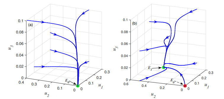
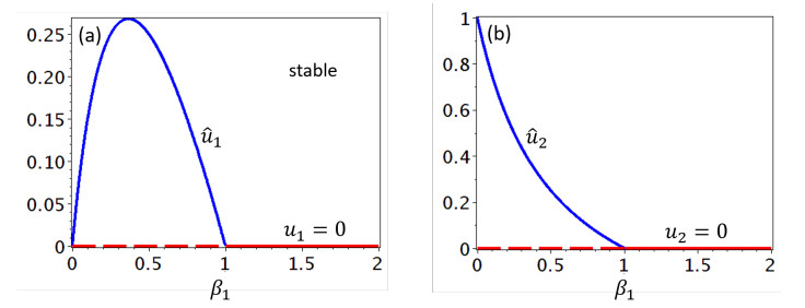
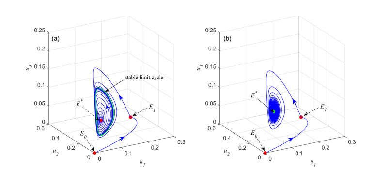
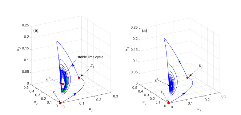
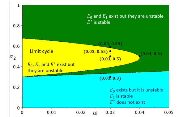
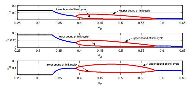
We consider a stage-structure Rosenzweig-MacArthur model describing the predator-prey interaction. Here, the prey population is divided into two sub-populations namely immature prey and mature prey. We assume that predator only consumes immature prey, where the predation follows the Holling type Ⅱ functional response. We perform dynamical analysis including existence and uniqueness, the positivity and the boundedness of the solutions of the proposed model, as well as the existence and the local stability of equilibrium points. It is shown that the model has three equilibrium points. Our analysis shows that the predator extinction equilibrium exists if the intrinsic growth rate of immature prey is greater than the death rate of mature prey. Furthermore, if the predation rate is larger than the death rate of predator, then the coexistence equilibrium exists. It means that the predation process on the prey determines the growing effects of the predator population. Furthermore, we also show the existence of forward and Hopf bifurcations. The dynamics of our system are confirmed by our numerical simulations.
Citation: Lazarus Kalvein Beay, Agus Suryanto, Isnani Darti, Trisilowati. Hopf bifurcation and stability analysis of the Rosenzweig-MacArthur predator-prey model with stage-structure in prey[J]. Mathematical Biosciences and Engineering, 2020, 17(4): 4080-4097. doi: 10.3934/mbe.2020226
We consider a stage-structure Rosenzweig-MacArthur model describing the predator-prey interaction. Here, the prey population is divided into two sub-populations namely immature prey and mature prey. We assume that predator only consumes immature prey, where the predation follows the Holling type Ⅱ functional response. We perform dynamical analysis including existence and uniqueness, the positivity and the boundedness of the solutions of the proposed model, as well as the existence and the local stability of equilibrium points. It is shown that the model has three equilibrium points. Our analysis shows that the predator extinction equilibrium exists if the intrinsic growth rate of immature prey is greater than the death rate of mature prey. Furthermore, if the predation rate is larger than the death rate of predator, then the coexistence equilibrium exists. It means that the predation process on the prey determines the growing effects of the predator population. Furthermore, we also show the existence of forward and Hopf bifurcations. The dynamics of our system are confirmed by our numerical simulations.

| [1] | A. J. Lotka, Elements of physical biology, Williams & Wilkins, Baltimore, 1925. |
| [2] | V. Volterra, Variazioni e fluttuazioni del numero d'individui in specie animali conviventi, Mem. Acad. Sci. Lincei, 2 (1926), 31-113. |
| [3] |
F. Wei, Q. Fu, Hopf bifurcation and stability for predator-prey systems with Beddington-DeAngelis type functional response and stage structure for prey incorporating refuge, Appl. Math. Model., 40 (2016), 126-134. doi: 10.1016/j.apm.2015.04.042

|
| [4] | M. Kot, Elements of mathematical ecology, Cambrige University Press, United Kingdom, 2001. |
| [5] | P. Turchin, Complex population dynamics: A theoritical/emphirical synthesis, Princeton University Press, United Kingdom, 2003. |
| [6] |
T. K. Kar, Stability analysis of a prey-predator model incorporating a prey refuge, Commun. Nonlin. Sci. Numer. Simul., 10 (2005), 681-691. doi: 10.1016/j.cnsns.2003.08.006
|
| [7] |
L. Chen, F. Chen, L. Chen, Qualitative analysis of a predator-prey model with Holling type Ⅱ functional response incorporating a constant prey refuge, Nonlin. Anal. Real World Appl., 11 (2010), 246-252. doi: 10.1016/j.nonrwa.2008.10.056
|
| [8] | E. Almanza-Vasquez, R. Ortiz-Ortiz, A. Marin-Ramirez, Bifurcations in the dynamics of Rosenzweig-MacArthur predator-prey model considering saturated refuge for the preys, Appl. Math. Sci., 150 (2015), 7475-7482. |
| [9] |
M. Moustofa, H. M. Mohd, A. I. Ismail, F. A. Abdullah, Dynamical analysis of a fractional order Rosenzweig-MacArthur model incorporating a prey refuge, Chaos Soliton. Fract., 109 (2018), 1-13. doi: 10.1016/j.chaos.2018.02.008
|
| [10] |
M. Javidi, N. Nyamoradi, Dynamic analysis of a fractional order prey-predator interaction with harvesting, Appl. Math. Model., 37 (2013), 8946-8956. doi: 10.1016/j.apm.2013.04.024
|
| [11] |
J. Wang, H. Fan, Dynamics in a Rosenzweig-MacArthur predator-prey system with quiescence, Discrete Contin. Dyn. Syst. -Ser. B, 21 (2016), 909-918. doi: 10.3934/dcdsb.2016.21.909
|
| [12] | F. M. Hilker, K. Schmitz, Disease-induced stabilization of predator-prey oscillations, J. Theor. Biol., 255 (2010), 299-306. |
| [13] | M. Moustofa, H. M. Mohd, A. I. Ismail, F. A. Abdullah, Dynamical analysis of a fractional-order eco-epidemiological model with disease in prey population, Adv. Differ. Equ., 1 (2020), 48. |
| [14] |
P Landi, F. Dercole, S. Rinaldi, Branching scenarios in eco-evolutionary prey-predator models, SIAM J. Appl. Math., 73(4), (2013) 1634-1658. doi: 10.1137/12088673X
|
| [15] |
P. Landi, J. R. Vonesh, C. Hui, Variability in life-history switch points across and within populations explained by Adaptive Dynamics, J. R. Soc. Interface, 15(148) (2018), 20180371. doi: 10.1098/rsif.2018.0371
|
| [16] |
P. Landi, C. Hui, U. Dieckmannd, Fisheries-induced disruptive selection, J. Theor. Biol., 365 (2015), 204-216. doi: 10.1016/j.jtbi.2014.10.017
|
| [17] |
X. Zhang, L. Chen, A. U. Newmann, The stage-structured predator-prey model and optimal harvesting policy, Math. Biosci., 168 (2000), 201-210. doi: 10.1016/S0025-5564(00)00033-X
|
| [18] | R. Xu, M. A. J. Chaplain, F. A. Davidson, Persistence and global stability of a ratio-dependent predator-prey model with stage structure, Appl. Math. Comput., 158 (2004), 729-744. |
| [19] | X.K. Sun, H.F. Huo, X.B. Zhang, A predator-prey model with functional response and stage structure for prey, Abstr. Appl. Anal., 1 (2012), 1-19. |
| [20] |
K. Chakraborty, S. Haldar, T. K. Kar, Global stability and bifurcation analysis of a delay induced prey-predator system with stage structure, Nonlin. Dyn., 73 (2013), 1307-1325. doi: 10.1007/s11071-013-0864-1
|
| [21] |
B. Dubey, A. Kumar, Dynamics of prey-predator model with stage structure in prey including maturation and gestation delays, Nonlin. Dyn., 96 (2019), 2653-2679. doi: 10.1007/s11071-019-04951-5
|
| [22] | F. Chen, Permanence of periodic Holling type predator-prey system with stage structure for prey, Appl. Math. Comput., 182 (2006), 1849-1860. |
| [23] |
W. Yang, X. Li, Z. Bai, Permanence of periodic Holling type-Ⅳ predator-prey system with stage structure for prey, Math. Comp. Model., 48 (2008), 677-684. doi: 10.1016/j.mcm.2007.11.003
|
| [24] |
S. Devi, Effects of prey refuge on a ratio-dependent predator-prey model with stage-structure of prey population, Appl. Math. Model., 37 (2013), 4337-4349. doi: 10.1016/j.apm.2012.09.045
|
| [25] | Y. Bai, Y. Li, Stability and Hopf bifurcation for a stage-structured predator-prey model incorporating refuge for prey and additional food for predator, Adv. Differ. Equ., 1 (2019), 42. |
| [26] |
S. K. G. Mortoja, P. Panja, S. K. Mondal, Dynamics of a predator-prey model with stage-structure on both species and anti-predator behavior, Inf. Med. Unlocked, 10 (2018), 50-57. doi: 10.1016/j.imu.2017.12.004
|
| [27] |
A. Apriyani, I. Darti, A. Suryanto, A stage-structure predator-prey model with ratio-dependent functional response and anti-predator, AIP Conf. Proc., 2084 (2019), 020002. doi: 10.1063/1.5094266
|
| [28] |
U. Salamah, A. Suryanto, M.K. Kusumawinahyu, Leslie-Gower predator-prey model with stage-structure, Beddington-DeAngelis functional response, and anti-predator behavior, AIP Conf. Proc., 2084 (2019), 020001. doi: 10.1063/1.5094265
|
| [29] |
S. Xu, Dynamics of a general prey-predator model with prey-stage structure and diffusive effects, Comp. Math. Appl., 68 (2014), 405-423. doi: 10.1016/j.camwa.2014.06.016
|
| [30] |
L.K. Beay, A. Suryanto, I. Darti, Trisilowati, Stability of a stage-structure Rosenzweig-MacArthur model incoporating Holling type-Ⅱ functional response, IOP Conf. Ser. Mater. Sci. Eng., 546 (2019), 052017. doi: 10.1088/1757-899X/546/5/052017
|
| [31] | C. J. Heij, C. F. E. Rompas, C. W. Moeliker, The biology of the Moluccan megapode Eulipoa wallacei (Aves, Galliformes, Megapodiidae) on Haruku and other Moluccan islands. Part 2, Final report, Deinsea, 3 (1997), 1-126. |
| [32] | S. Wang, Research on the suitable living environment of the Rana temporaria chensinensis larva, Chinese J. Zool., 32(1) (1997), 38-41 |
| [33] | J. D. Murray, Mathematical Biology: I. An Introduction, Springer Verlag, New York, 2002. |
Figures(6) / Tables(1)

Lazarus Kalvein Beay, Agus Suryanto, Isnani Darti, Trisilowati. Hopf bifurcation and stability analysis of the Rosenzweig-MacArthur predator-prey model with stage-structure in prey[J]. Mathematical Biosciences and Engineering, 2020, 17(4): 4080-4097. doi: 10.3934/mbe.2020226


 DownLoad: