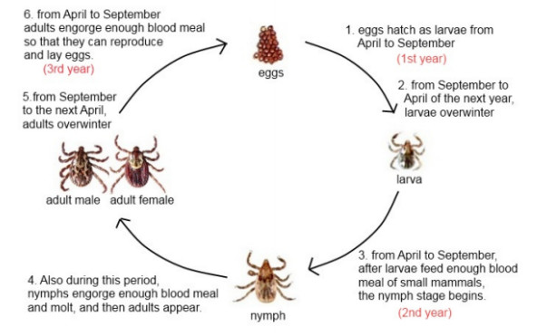
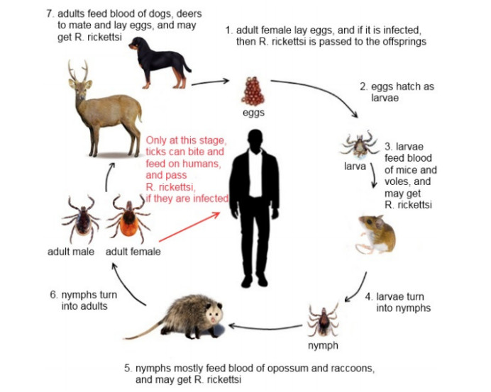
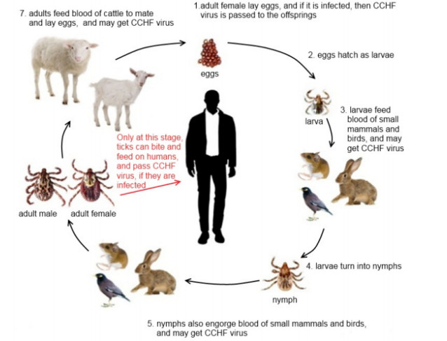
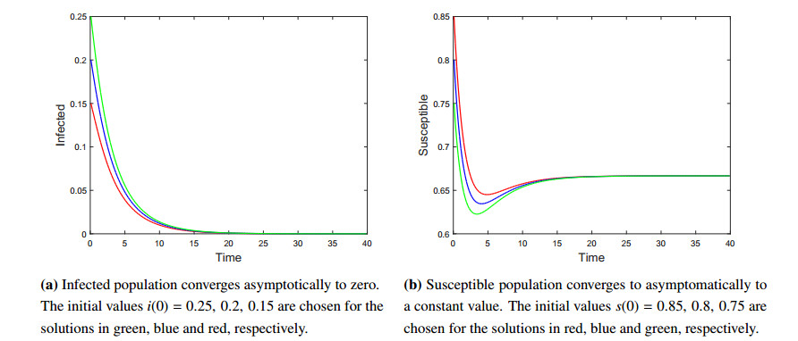
A tick-borne disease model is considered with nonlinear incidence rate and piecewise constant delay of generalized type. It is known that the tick-borne diseases have their peak during certain periods due to the life cycle of ticks. Only adult ticks can bite and transmit disease. Thus, we use a piecewise constant delay to model this phenomena. The global asymptotic stability of the disease-free and endemic equilibrium is shown by constructing suitable Lyapunov functions and Lyapunov-LaSalle technique. The theoretical findings are illustrated through numerical simulations.
Citation: Ardak Kashkynbayev, Daiana Koptleuova. Global dynamics of tick-borne diseases[J]. Mathematical Biosciences and Engineering, 2020, 17(4): 4064-4079. doi: 10.3934/mbe.2020225
A tick-borne disease model is considered with nonlinear incidence rate and piecewise constant delay of generalized type. It is known that the tick-borne diseases have their peak during certain periods due to the life cycle of ticks. Only adult ticks can bite and transmit disease. Thus, we use a piecewise constant delay to model this phenomena. The global asymptotic stability of the disease-free and endemic equilibrium is shown by constructing suitable Lyapunov functions and Lyapunov-LaSalle technique. The theoretical findings are illustrated through numerical simulations.

| [1] |
R. Jennings, Y. Kuang, H. R. Thieme, J. Wu, X. Wu, How ticks keep ticking in the adversity of host immune reactions, J. Math. Biol., 78 (2019), 1331-1364. doi: 10.1007/s00285-018-1311-1

|
| [2] | Centers for Disease Control and Prevention, Epidemiology and Statistics-Rocky Mountain Spotted Fever (RMSF). Available from: https://www.cdc.gov/rmsf/stats. |
| [3] | T. Nurmakhanov, Y. Sansyzbaev, B. Atshabar, P. Deryabin, S. Kazakov, A. Zholshorinov, et al., Crimean-Congo haemorrhagic fever virus in Kazakhstan (1948-2013), Int. J. Infect. Dis., 38 (2015), 19-23. |
| [4] | B. Knust, Z. B. Medetov, K. B. Kyraubayev, Y. Bumburidi, B. R. Erickson, A. MacNeil, et al., Crimean-Congo Hemorrhagic Fever, Kazakhstan, 2009-2010, Emerg. Infect. Dis., 18 (2012), 643-645. |
| [5] | L. J. S. Allen, Some discrete-time SI, SIR, and SIS epidemic models, Math. Biosci., 124 (1994), 83-105. |
| [6] |
I. Győri, On approximation of the solutions of delay differential equations by using piecewise constant arguments, Int. J. Math. Math. Sci., 14 (1991), 111-126. doi: 10.1155/S016117129100011X
|
| [7] |
I. Győri, F. Hartung, On numerical approximation using differential equations with piecewiseconstant arguments, Period. Math. Hung., 56 (2008), 55-69. doi: 10.1007/s10998-008-5055-5
|
| [8] |
S. Kartal, F. Gurcan, Discretization of conformable fractional differential equations by a piecewise constant approximation, Int. J. Comput. Math., 96 (2019), 1849-1860. doi: 10.1080/00207160.2018.1536782
|
| [9] | S. Busenberg, K. L. Cooke, Models of vertically transmitted diseases with sequential-continuous dynamics, in Nonlinear Phenomena in Mathematical Sciences (eds. V. Lakshmikantham), Academic Press, (1984), 265-297. |
| [10] | K. L. Cooke, J. Wiener, Retarded differential equations with piecewise constant delays, J. Math. Anal. Appl. 99 (1984), 265-297. |
| [11] |
S. M. Shah, J. Wiener, Advanced differential equations with piecewise constant argument deviations, Int. J. Math. Math. Sci., 6 (1983), 671-703. doi: 10.1155/S0161171283000599
|
| [12] | Y. Muroya, Persistence, contractivity and global stability in logistic equations with piecewise constant delays, J. Math. Anal. Appl., 270 (2002), 602-635. |
| [13] | D. Aruǧaslan, A. Özer, Stability analysis of a predator-prey model with piecewise constant argument of generalized type using Lyapunov functions, J. Math. Sci., 203 (2014), 297-305. |
| [14] |
Q. Xi, Global Exponential Stability of Cohen-Grossberg Neural Networks with Piecewise Constant Argument of Generalized Type and Impulses, Neural Comput., 28 (2016), 229-255. doi: 10.1162/NECO_a_00797
|
| [15] |
F. Gurcan, S. Kartal, I. Ozturk, F. Bozkurt, Stability and bifurcation analysis of a mathematical model for tumor-immune interaction with piecewise constant arguments of delay, Chaos Solit. Fract., 68 (2014), 169-179. doi: 10.1016/j.chaos.2014.08.001
|
| [16] |
I. Ozturk, F. Bozkurt, F. Gurcan, Stability analysis of a mathematical model in a microcosm with piecewise constant arguments, Math. Biosci., 240 (2012), 85-91. doi: 10.1016/j.mbs.2012.08.003
|
| [17] | X. Liu, P. Stechlinski, Infectious Disease Modeling: A Hybrid System Approach, Springer, (2017). |
| [18] | University of Maine Cooperative Extension, American Dog Tick, Cooperative Extension: Tick Lab. Available from: https://extension.umaine.edu/ticks/maine-ticks/american-dog-tick. |
| [19] | S. Aslam, M. S. Latif, M. Daud, Z. U. Rahman, B. Tabassum, M. S. Riaz, et al., Crimean-Congo Hemorrhagic Fever: Risk Factors And Control Measures For The Infection Abatement, Biomed. Rep., 4 (2015), 15-20. |
| [20] | M. Akhmet, Nonlinear hybrid continuous/discrete-time models, Atlantis Press, (2011). |
| [21] |
M. Akhmet, D. Arugaslan, Lyapunov-Razumikhin method for differential equations with piecewise constant argument, Discrete Cont. Dyn. A, 25 (2009), 457-466. doi: 10.3934/dcds.2009.25.457
|
| [22] |
A. Korobeinikov, Lyapunov functions and global stability for SIR and SIRS epidemiological models with non-linear transmission, Bull. Math. Bio., 68 (2006), 615-626. doi: 10.1007/s11538-005-9037-9
|
| [23] | A. Korobeinikov, P. K. Maini, A Lyapunov function and global properties for SIR and SEIR epidemiological models with nonlinear incidence, Math. Biosci. Eng., 1 (2006), 57-60. |
| [24] |
E. Beretta, T. Hara, W. Ma, Y. Takeuchi, Global asymptotic stability of an SIR epidemic model with distributed time delay, Nonlinear Anal. Theory Methods Appl., 47 (2001), 4107-4115. doi: 10.1016/S0362-546X(01)00528-4
|
| [25] |
G. Huang, Y. Takeuchi, W. Ma, D. Wei, Global Stability for Delay SIR and SEIR Epidemic Models with Nonlinear Incidence Rate, Bull. Math. Bio., 72 (2010), 1192-1207. doi: 10.1007/s11538-009-9487-6
|
| [26] |
P. Van den Driessche, J. Watmough, Reproduction numbers and sub-threshold endemic equilibria for compartmental models of disease transmission, Math. Biosci., 180 (2002), 29-48. doi: 10.1016/S0025-5564(02)00108-6
|
| [27] |
A. Korobeinikov, P. K. Maini, Nonlinear incidence and stability of infectious disease models, Math. Med. Biol., 22 (2005), 113-128. doi: 10.1093/imammb/dqi001
|
| [28] | J. K. Hale, S. M. V. Lunel, Introduction to Functional Differential Equations, Springer, (1993). |
| [29] | Y. Kuang, Delay Differential Equations with Applications in Population Dynamics, Academic Press, (1993). |
| [30] |
Y. Pei, L. Chen, Q. Zhang, C. Li, Extinction and permanence of one-prey multi-predators of Holling type II function response system with impulsive biological control, J. Theor. Bio., 235 (2005), 495-503. doi: 10.1016/j.jtbi.2005.02.003
|
| [31] |
F. A. Rihan, S. Lakshmanan, A. H. Hashish, R. Rakkiyappan, E. Ahmed, Fractional-order delayed predator-prey systems with Holling type-II functional response, Nonlinear Dyn., 80 (2015), 777-789. doi: 10.1007/s11071-015-1905-8
|
| [32] |
X. Wu, V. R. Duvvuri, Y. Lou, N. H. Ogden, Y. Pelcat, J. Wu, Developing a temperature-driven map of the basic reproductive number of the emerging tick vector of Lyme disease Ixodes scapularis in Canada, J. Theor. Biol., 319 (2013), 50-61. doi: 10.1016/j.jtbi.2012.11.014
|
| [33] |
N. A. Hartemink, S. E. Randolph, S. A. Davis, J. A. P. Heesterbeek, The basic reproduction number for complex disease systems: Defining R0 for tick-borne infections, Am. Nat., 171 (2008), 743-754. doi: 10.1086/587530
|

Figures(7) / Tables(1)

Ardak Kashkynbayev, Daiana Koptleuova. Global dynamics of tick-borne diseases[J]. Mathematical Biosciences and Engineering, 2020, 17(4): 4064-4079. doi: 10.3934/mbe.2020225


 DownLoad: