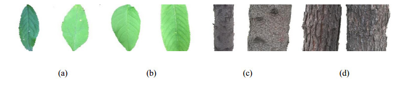
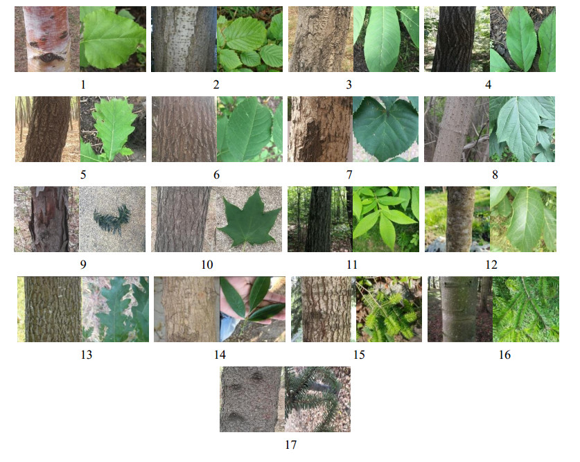
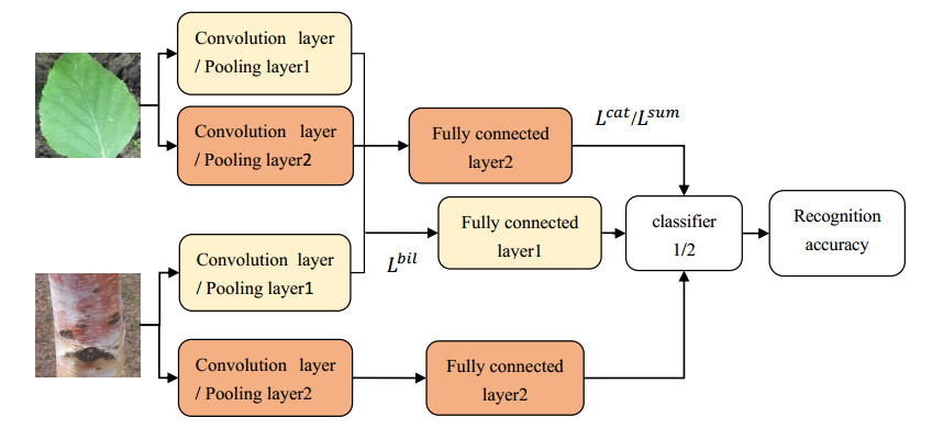
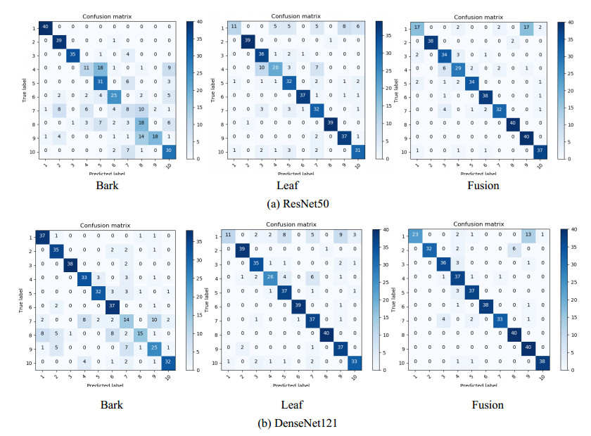
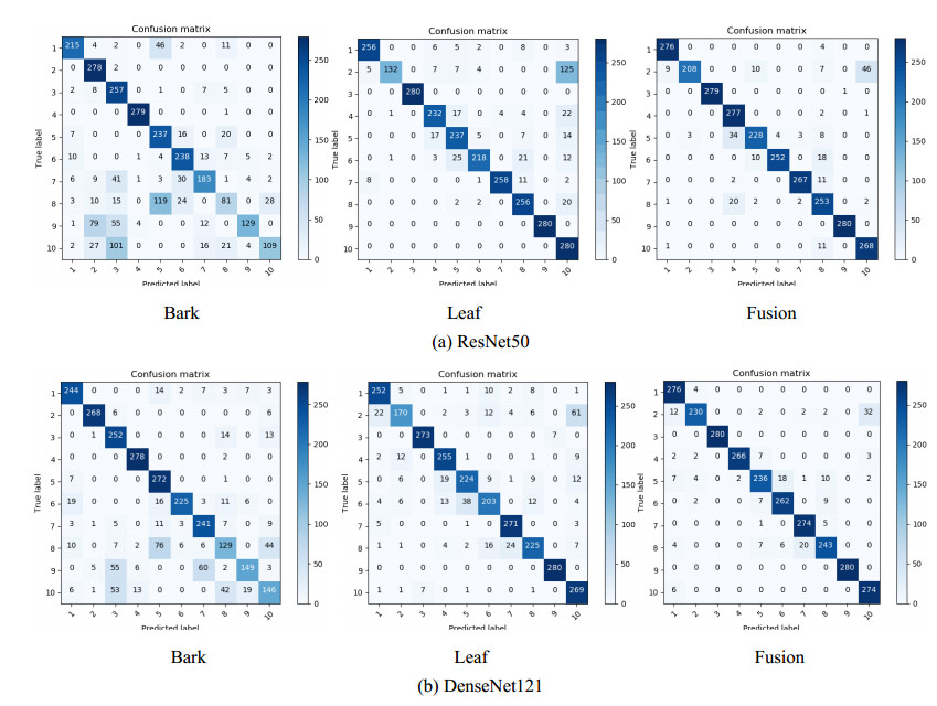
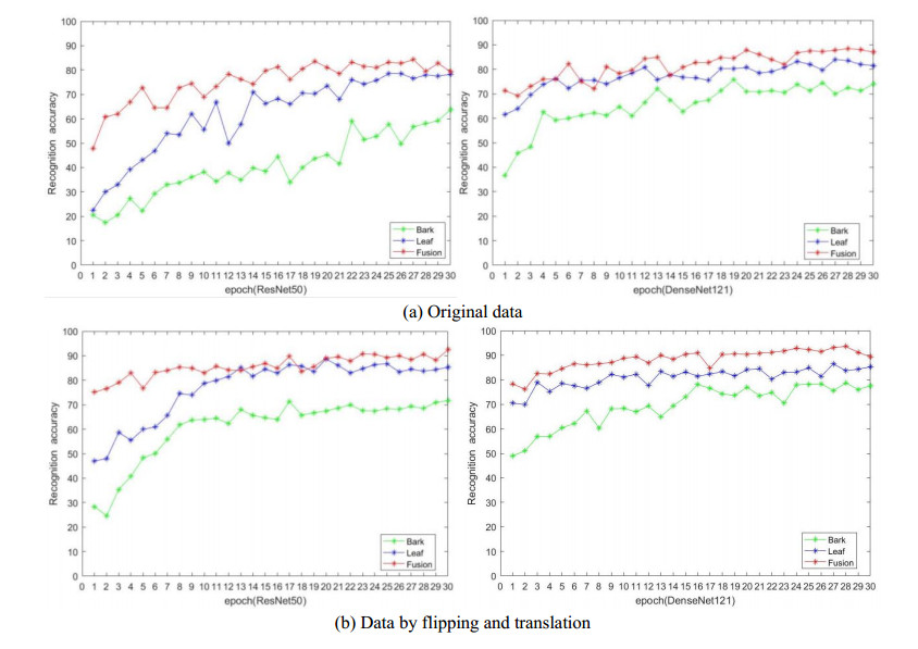
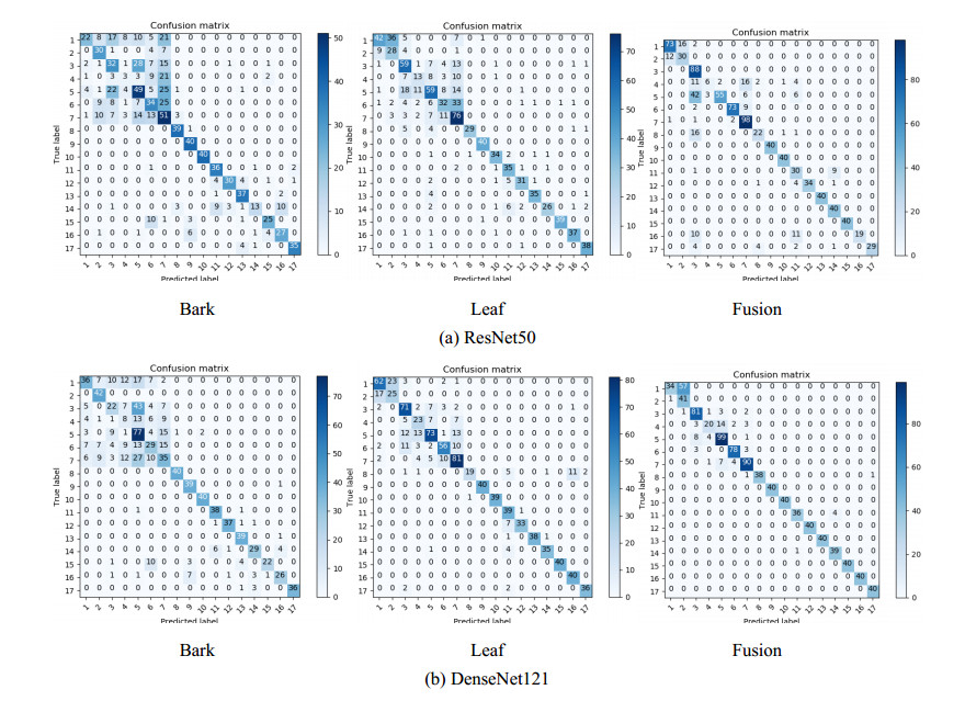
For trees, leaves are often used for identification, but the shape of leaves changes greatly, bark will be another identifying feature. However, it is difficult to recognize by a single organ when there are intra class differences and inter class similarities between leaves or bark. So we fuse features of leaf and bark. Firstly, we collected 17 species of leaves and bark of trees through field shooting and web crawling. Then propose a method of combining convolution neural network (CNN) with cascade fusion, additive fusion algorithm, bilinear fusion and score level fusion. Finally, the features extracted from the leaves and bark are fused in the ReLu layer and Fully connected layer. The method was compared with single organ recognition, Support Vector Machines (SVM), and existing fusion methods, results show that the two organ fusion method proposed are better than the other recognition methods, and recognition accuracy is 87.86%. For similar trees, when it is impossible to accurately determine its species by a single organ, the fusion of two organs can effectively improve this situation.
Citation: Yafeng Zhao, Xuan Gao, Junfeng Hu, Zhen Chen. Tree species identification based on the fusion of bark and leaves[J]. Mathematical Biosciences and Engineering, 2020, 17(4): 4018-4033. doi: 10.3934/mbe.2020222
For trees, leaves are often used for identification, but the shape of leaves changes greatly, bark will be another identifying feature. However, it is difficult to recognize by a single organ when there are intra class differences and inter class similarities between leaves or bark. So we fuse features of leaf and bark. Firstly, we collected 17 species of leaves and bark of trees through field shooting and web crawling. Then propose a method of combining convolution neural network (CNN) with cascade fusion, additive fusion algorithm, bilinear fusion and score level fusion. Finally, the features extracted from the leaves and bark are fused in the ReLu layer and Fully connected layer. The method was compared with single organ recognition, Support Vector Machines (SVM), and existing fusion methods, results show that the two organ fusion method proposed are better than the other recognition methods, and recognition accuracy is 87.86%. For similar trees, when it is impossible to accurately determine its species by a single organ, the fusion of two organs can effectively improve this situation.

| [1] | P. Yuan, W. Li, S. Ren, H. Xu, Recognition for flower type and variety of chrysanthemum with convolutional neural network, Trans. Chin. Soc. Agric. Eng., 34 (2018), 152-158. |
| [2] | G. Xuan, Y. Zhao, Q. Xiong, Z. Chen, Identification of Tree Species Based on Transfer Learning, For. Eng., 35 (2019), 68-75. |
| [3] |
X. Zhu, M. Zhu, H. Ren, Method of plant leaf recognition based on improved deep convolutional neural network, Cognit. Syst. Res., 52 (2018), 223-233. doi: 10.1016/j.cogsys.2018.06.008

|
| [4] | H. Feng, M. Hu, Y. Yang, K. Xia, Tree Species Recognition Based on Overall Tree Image and Ensemble of Transfer Learning, Trans. Chin. Soc. Agric. Mach., 8 (2019), 235-279. |
| [5] | L. Bi, Plant species recognition based on leaf image algorithm, Acta Agric. Zhejiangensis, 29 (2017), 2142-2148. |
| [6] | P. Mittal, M. Kansal, H. K. Jhajj, Combined Classifier for Plant Classification and Identification from Leaf Image Based on Visual Attributes, 2018 International Conference on Intelligent Circuits and Systems, 2018. Available from: https://ieeexplore.ieee.org/abstract/document/8479567. |
| [7] |
M. Kumar, S. Gupta, X. Gao, A. Singh, Plant Species Recognition Using Morphological Features and Adaptive Boosting Methodology, IEEE Access, 7 (2019), 163912-163918. doi: 10.1109/ACCESS.2019.2952176
|
| [8] |
N. Liu, J. Kan, Improved deep belief networks and multi-feature fusion for leaf identification, Neurocomputing, 216 (2016), 460-467. doi: 10.1016/j.neucom.2016.08.005
|
| [9] | X. Zhang, Y. Liu, H. Lin, Y. Liu, Research on SVM Plant Leaf Identification Method Based on CSA, International Conference of Pioneering Computer Scientists, Engineers and Educators, 2016. Available from: https://link.springer.com/chapter/10.1007/978-981-10-2098-8_20. |
| [10] | T. P. Kumar, M. V. P. Reddy, P. K. Bora, Leaf Identification Using Shape and Texture Features, Proceedings of international conference on computer vision and image processing, 2017. Available from: https://link.springer.com/chapter/10.1007/978-981-10-2107-7_48. |
| [11] | S. Boudra, I. Yahiaoui, A. Behloul, Statistical Radial Binary Patterns (SRBP) for Bark Texture Identification, International Conference on Advanced Concepts for Intelligent Vision Systems, 2017. Available from: https://link.springer.com/chapter/10.1007/978-3-319-70353-4_9. |
| [12] | J. Chaki, R. Parekh, S. Bhattacharya, Plant leaf classification using multiple descriptors: A hierarchical approach, J. King Saud Univ., 2018 (2018). |
| [13] | J. Chaki, N. Dey, L. Moraru, F. Shi, Fragmented plant leaf recognition: Bag-of-features, fuzzy-color and edge-texture histogram descriptors with multi-layer perceptron. Optik, 181 (2019), 639-650. |
| [14] | S. L. Pimm, S. Alibhai, R. Berg, A. Dehgan, C. Giri, Z. Jewell, et al., Emerging technologies to conserve biodiversity. Trends. Ecol. Evol., 30 (2015), 685-696. |
| [15] | M. Carpentier, P. Giguère, J. Gaudreault, Tree Species Identification from Bark Images Using Convolutional Neural Networks, 2018 IEEE/RSJ International Conference on Intelligent Robots and Systems, 2018. Available from: https://ieeexplore.ieee.org/abstract/document/8593514/. |
| [16] | J. Zheng, X. Wang, T. Wang, Research on image recognition of five bark texture images based on deep learning, J. Beijing For. Univ., 41 (2019), 150-158. |
| [17] | S. Razavi, H. Yalcin, Using convolutional neural networks for plant classification, 2017 25th Signal Processing and Communications Applications Conference, 2017. Available from: https://ieeexplore.ieee.org/abstract/document/7960654. |
| [18] | H. Zhou, C. Yan, H. Huang, Tree Species Identification Based on Convolutional Neural Network, 2016 8th International Conference on Intelligent Human-Machine Systems and Cybernetics (IHMSC), 2016. Available from: https://ieeexplore.ieee.org/abstract/document/7783797/. |
| [19] | X. Zhang, J. Chen, J. ZhuGe, L. Yu, Deep Learning Based Fast Plant Image Recognition, J. East China Univ. Sci. Technol., 44 (2018), 105-113. |
| [20] | H. Zhang, G. He, J. Peng, Z. Kuang, J. Fan, Deep Learning of Path-Based Tree Classifiers for Large-Scale Plant Species Identification, 2018 IEEE Conference on Multimedia Information Processing and Retrieval (MIPR), 2018. Available from: https://ieeexplore.ieee.org/abstract/document/8396969. |
| [21] | P. Guo, Q. Gao, A multi-organ plant identification method using convolutional neural networks, 2017 8th IEEE International Conference on Software Engineering and Service Science (ICSESS), 2017. Available from: https://ieeexplore.ieee.org/abstract/document/8342935. |
| [22] |
S. Bertrand, R. B. Ameur, G. Cerutti, D. Coquin, L. Valet, L. Tougne, Bark and leaf fusion systems to improve automatic tree species recognition, Ecol. Inform., 46 (2018), 57-73. doi: 10.1016/j.ecoinf.2018.05.007
|
| [23] | M. Rzanny, P. Mä der, A. Deggelmann, M. Chen, J. Wä ldchen, Flowers, leaves or both? How to obtain suitable images for automated plant identification, Plant Methods, 15 (2019), 77. |
| [24] | H. Goë au, P. Bonnet, A. Joly, V. Bakić, J. Barbe, I. Yahiaoui, et al., Pl@ntNet mobile app, Proceedings of the 21st ACM international conference on Multimedia, 2013. Available from: https://dl.acm.org/doi/abs/10.1145/2502081.2502251. |
| [25] | iNaturalist, https://www.inaturalist.org/, Accessed 15 July 2019. |
| [26] | J. Champ, T. Lorieul, M. Servajean, A. Joly, A comparative study of fine-grained classification methods in the context of the LifeCLEF plant identification challenge 2015, CLEF, 2015 (2015). |
| [27] |
S. H. Lee, C. S. Chan, P. Remagnino, Multi-organ plant classification based on convolutional and recurrent neural networks, IEEE Trans. Image Process., 27 (2018), 4287-4301. doi: 10.1109/TIP.2018.2836321
|
| [28] | A. Joly, P. Bonnet, H. Goë au, J. Barbe, S. Selmi, J. Champ, et al., A look inside the pl@ntnet experience, Multimed Syst., 22 (2016), 751-766. |
| [29] | K. He, X. Zhang, S. Ren, J. Sun, Deep residual learning for image recognition, Proceedings of the IEEE conference on computer vision and pattern recognition, 2016. Available from: http://openaccess.thecvf.com/content_cvpr_2016/. |
| [30] | G. Huang, Z. Liu, L. Maaten, K. Q. Weinberger, Densely connected convolutional networks, Proceedings of the IEEE conference on computer vision and pattern recognition, 2017. Available from: http://openaccess.thecvf.com/content_cvpr_2017/. |
| [31] | W. B. Liu, Z. Y. Zou, W. W. Xing, Feature Fusion Methods in Pattern Classification, J. Beijing Univ. Posts Telecommun., 4 (2017), 5-12. |
| [32] | A He, X Tian, Multi-organ plant identification with multi-column deep convolutional neural networks, 2016 IEEE international conference on systems, man, and cybernetics (SMC), 2016. Available from: https://ieeexplore.ieee.org/abstract/document/7844537. |
Figures(7) / Tables(8)

Yafeng Zhao, Xuan Gao, Junfeng Hu, Zhen Chen. Tree species identification based on the fusion of bark and leaves[J]. Mathematical Biosciences and Engineering, 2020, 17(4): 4018-4033. doi: 10.3934/mbe.2020222


 DownLoad: