Minimally invasive treatment of calcaneal fractures via the sinus tarsi approach based on a 3D printing technique

Lufeng Yao; Haiqing Wang; Feng Zhang; Liping Wang; Jianghui Dong; Lufeng Yao; Haiqing Wang; Feng Zhang; Liping Wang; Jianghui Dong

doi:10.3934/mbe.2019076

Mathematical Biosciences and Engineering

2019, Volume 16, Issue 3: 1597-1610. doi: 10.3934/mbe.2019076

Previous Article Next Article

Research article Special Issues

Minimally invasive treatment of calcaneal fractures via the sinus tarsi approach based on a 3D printing technique

1.
Department of Foot and Ankle Surgery, Ningbo No. 6 Hospital, Ningbo, 315040, China
2.
Department of Hand Surgery, Department of Plastic Reconstructive Surgery, Ningbo No. 6 Hospital, Ningbo, 315040, China
3.
School of Pharmacy and Medical Sciences, University of South Australia, Adelaide, SA 5001, Australia

Received: 22 December 2018 Accepted: 27 January 2019 Published: 26 February 2019

The sinus tarsi approach can be used for a limited exposure of the calcaneal fracture site. The reduction of the posterior articular surface, the shape of the calcaneus, the precise placement of the sustentacular screw (SS), the posterior articular surface screw of the calcaneal (PASS), and the long axis screw of the calcaneal (LAS) are still challenging. To that end, we proposed a minimally invasive technique for the treatment of calcaneal fractures via the sinus tarsi approach in combination with a three-dimensional (3D) printing technique. First, a 3D reconstructed model of the bilateral calcanei was obtained according to the computed tomography (CT) scan data and was used to simulate the placement of screws and acquire the screw trajectory parameters. Next, using 3D printing, a model of the calcaneus was printed, and the minimally invasive steel plate was pre-shaped to fit the lateral wall of the model. Finally, a total of 25 patients underwent this procedure. The results showed significant accuracy improvement in terms of the SS, PASS and LAS placement and in terms of the parameters including Bohler's angle, Gissane's angle, and the calcaneal width. In this work, the technique of the personalized minimally invasive treatment of calcaneal fractures improved the accuracy of screw placement (SP) and the reduction rate of posterior articular surface, improved the shape of the calcaneus, and increased the precision of the minimally invasive treatment of calcaneal fractures via the sinus tarsi approach.

Keywords:

Citation: Lufeng Yao, Haiqing Wang, Feng Zhang, Liping Wang, Jianghui Dong. Minimally invasive treatment of calcaneal fractures via the sinus tarsi approach based on a 3D printing technique[J]. Mathematical Biosciences and Engineering, 2019, 16(3): 1597-1610. doi: 10.3934/mbe.2019076

Related Papers:

[1]	Ahmed Abul Hasanaath, Abdul Sami Mohammed, Ghazanfar Latif, Sherif E. Abdelhamid, Jaafar Alghazo, Ahmed Abul Hussain . Acute lymphoblastic leukemia detection using ensemble features from multiple deep CNN models. Electronic Research Archive, 2024, 32(4): 2407-2423. doi: 10.3934/era.2024110
[2]	Abul Bashar . Employing combined spatial and frequency domain image features for machine learning-based malware detection. Electronic Research Archive, 2024, 32(7): 4255-4290. doi: 10.3934/era.2024192
[3]	Yazhuo Fan, Jianhua Song, Yizhe Lu, Xinrong Fu, Xinying Huang, Lei Yuan . DPUSegDiff: A Dual-Path U-Net Segmentation Diffusion model for medical image segmentation. Electronic Research Archive, 2025, 33(5): 2947-2971. doi: 10.3934/era.2025129
[4]	Kuntha Pin, Jung Woo Han, Yunyoung Nam . Retinal diseases classification based on hybrid ensemble deep learning and optical coherence tomography images. Electronic Research Archive, 2023, 31(8): 4843-4861. doi: 10.3934/era.2023248
[5]	Mashael S. Maashi, Yasser Ali Reyad Ali, Abdelwahed Motwakel, Amira Sayed A. Aziz, Manar Ahmed Hamza, Amgad Atta Abdelmageed . Anas platyrhynchos optimizer with deep transfer learning-based gastric cancer classification on endoscopic images. Electronic Research Archive, 2023, 31(6): 3200-3217. doi: 10.3934/era.2023162
[6]	Jinjiang Liu, Yuqin Li, Wentao Li, Zhenshuang Li, Yihua Lan . Multiscale lung nodule segmentation based on 3D coordinate attention and edge enhancement. Electronic Research Archive, 2024, 32(5): 3016-3037. doi: 10.3934/era.2024138
[7]	Zengyu Cai, Liusen Xu, Jianwei Zhang, Yuan Feng, Liang Zhu, Fangmei Liu . ViT-DualAtt: An efficient pornographic image classification method based on Vision Transformer with dual attention. Electronic Research Archive, 2024, 32(12): 6698-6716. doi: 10.3934/era.2024313
[8]	Yanxia Sun, Tianze Xu, Jing Wang, Jinke Wang . DST-Net: Dual self-integrated transformer network for semi-supervised segmentation of optic disc and optic cup in fundus image. Electronic Research Archive, 2025, 33(4): 2216-2245. doi: 10.3934/era.2025097
[9]	Yixin Sun, Lei Wu, Peng Chen, Feng Zhang, Lifeng Xu . Using deep learning in pathology image analysis: A novel active learning strategy based on latent representation. Electronic Research Archive, 2023, 31(9): 5340-5361. doi: 10.3934/era.2023271
[10]	Tej Bahadur Shahi, Cheng-Yuan Xu, Arjun Neupane, Dayle B. Fleischfresser, Daniel J. O'Connor, Graeme C. Wright, William Guo . Peanut yield prediction with UAV multispectral imagery using a cooperative machine learning approach. Electronic Research Archive, 2023, 31(6): 3343-3361. doi: 10.3934/era.2023169

Abstract

1. Introduction

The data generated by the daily work environment are more complex in nature at present, and therefore many lifetime models have been listed in the literature to analyze and evaluate these data. Determining which probability distribution should be adopted to make inferences from the data under study is a very important problem in statistics. For these reasons, great efforts have been spent over the years in developing large categories of distributions along with relevant statistical methodologies. See, for instance, El-Gohary et al. ^[1], Saboor et al. ^[2], Jia et al. ^[3], Fernandez ^[4], Alizadeh et al. ^[5], Kumar et al. ^[6], and references cited therein. Nedjar and Zeghdoudi ^[7] proposed a mixture of gamma( $2, \tau$ ) and Lindley( $\varepsilon$ ) (MGL) distributions. The probability density function (PDF) of the MGL distribution can be expressed as

$\begin{equation} g(x;\varepsilon, \tau) = \frac{\tau^{2}}{\varepsilon(1+\tau)}\left( \left[ \tau\varepsilon+\varepsilon-\tau\right] x+1\right) e^{-\tau x} ;\ x > 0, \varepsilon > 0, \tau > 0. \end{equation}$

(1.1)

Unfortunately, Eq (1.1) is not a proper PDF. Messaadia and Zeghdoudi ^[8] corrected the parameter space to be $\varepsilon\geq\frac{\tau }{1+\tau}$ and $\tau > 0$ , and consequently the modified PDF of the MGL model can be written as

$\begin{equation} f(x;\varepsilon, \tau) = \frac{\tau^{2}}{\varepsilon(1+\tau)}\left( \left[ \tau\varepsilon+\varepsilon-\tau\right] x+1\right) e^{-\tau x} ;\ x > 0, \varepsilon\geq\frac{\tau}{1+\tau}, \tau > 0. \end{equation}$

(1.2)

The survival function (SF) corresponding to Eq (1.2) can be formulated as

$\begin{equation} S(x;\varepsilon, \tau) = \frac{(\tau x+1)(\tau\varepsilon+\varepsilon-\tau)+\tau }{\varepsilon(1+\tau)}e^{-\tau x};\ x > 0, \varepsilon\geq\frac{\tau}{1+\tau }, \tau > 0. \end{equation}$

(1.3)

The quantile function (QF) is

$\begin{equation} Q_{X}(u) = \left\{ \begin{array} [c]{l} -\frac{\varepsilon(1+\tau)}{\tau\left[ \varepsilon\left( 1+\tau\right) -\tau\right] }-\frac{1}{\tau}W_{-1}\left( \frac{\varepsilon\left( 1+\tau\right) (u-1)}{\varepsilon\left( 1+\tau\right) -\tau}e^{-\frac {\varepsilon(1+\tau)}{\varepsilon\left( 1+\tau\right) -\tau}}\right) ;\ \varepsilon > \frac{\tau}{1+\tau}\\ \\ \frac{-\ln(1-u)}{\tau} \ \ \ \ \ \ \ \ \ \ \ \ \ \ \ \ \ \ \ \ \ \ \ \ \ \ \ \ \ \ \ \ \ \ \ \ \ \ \ \ \ \ \ \ \ \ \ \ \ ;\ \ \ \varepsilon = \frac{\tau}{1+\tau}, \end{array} \right. \end{equation}$

(1.4)

where $W_{-1}\$ denotes the negative branch of the Lambert $W$ function, and $\frac{-\ln(1-u)}{\tau}$ is the QF of the exponential model. Sometimes, survival trials produce data that are discrete in nature either because of the limitations of the measuring instruments or their inherent characteristics. The study and analysis of counting data plays an important role in many fields of applied sciences, such as economics, engineering, marketing, medicine, and insurance. Counting datasets are often modeled utilizing the Poisson model. However, the Poisson model cannot handle hyper-scattered datasets. Therefore, it is reasonable to model such cases via an appropriate discrete distribution. Discretization of a continuous distribution can be created by using several methods. The most widely utilized technique is the survival discretization approach. For a given continuous random variable $X$ with SF $S(x; \xi ) = \Pr(X > x)$ , we can obtain the discretized version as

$\begin{equation} \Pr(X = x) = S(x;\xi )-S(x+1;\xi );\ x = 0, 1, 2, 3, .... \end{equation}$

(1.5)

For more details, Roy ^[9]. This technique has received a lot of attention in recent years. See, for instance, Gómez-Déniz and Calderín-Ojeda ^[10], Bebbington et al. ^[11], Nekoukhou et al. ^[12], Alamatsaz et al. ^[13], El-Morshedy et al. ^[14], Gillariose et al. ^[15], Singh et al. ^[16,17], Eliwa and El-Morshedy ^[18], Altun et al. ^[19] and references cited therein. In this paper, a discrete distribution MGL (DsMGL) will be discussed from the point of view of reliability and ordered statistics theoretically and practically to analyze extreme and outliers' notes. This is because in El-Morshedy et al. ^[20], simple statistical characteristics and a regression model were presented only in a small whole sample (outliers were not included). Further, the previous paper ignored the reliability, order statistics, and L-moments measures which can be applied in the fields of biomedicine and engineering. Given the importance of reliability and structured statistical measures, the authors sought to discuss neglected characteristics as well as model extreme and outliers' observations. Thus, the motives for this study can be summarized as follows: to formulate statistical characteristics as closed forms; to model dispersed-positively-skewed real data under extreme and outliers' observations; to provide a consistently better fit than other discrete models known in the current statistical literature, especially over-dispersed models; and to prove that the proposed model can be applied to discuss zero-inflated observations.

The article is organized as follows. In Section 2, the DsMGL distribution is proposed. Various properties are derived in Sections 3 and 4. In Section 5, the DsMGL parameters are estimated by utilizing the maximum likelihood approach. Simulation study is discussed in Section 6. In Section 7, three real data sets are analyzed. Finally, some conclusions and future work are listed in Section 8.

2. Discrete analogue of MGL distribution

Recall Eq (1.3), and the SF of the DsMGL distribution can be expressed as

$\begin{equation} S(x;\varepsilon, \delta) = \frac{(1-\ln\delta^{x+1})(\varepsilon-\varepsilon \ln\delta+\ln\delta)-\ln\delta}{\varepsilon(1-\ln\delta)}\delta^{x+1};\ x\in \mathbb{N} _{0}, \end{equation}$

(2.1)

where $\varepsilon\geq\frac{-\ln\delta}{1-\ln\delta}$ , $0 < e^{-\tau} = \delta < 1,$ and $\mathbb{N} _{0} = \left\{ 0, 1, 2, 3, ...\right\}$ . The corresponding PMF to Eq (2.1) can be introduced as

$\begin{equation} P_{x}(x;\varepsilon, \delta) = \frac{\delta^{x}}{1-\ln\delta}\left\{ 1-\delta-\ln\delta\left[ 1+x-\delta(x+2)\right] +(1-\frac{1}{\varepsilon })(\ln\delta)^{2}\left[ x-\delta(x+1)\right] \right\} ;\ x\in \mathbb{N} _{0}. \end{equation}$

(2.2)

The CDF can be reported as

$\begin{equation} F(x;\varepsilon, \delta) = 1-\frac{(1-\ln\delta^{x+1})(\varepsilon-\varepsilon \ln\delta+\ln\delta)-\ln\delta}{\varepsilon(1-\ln\delta)}\delta^{x+1};\ x\in \mathbb{N} _{0}. \end{equation}$

(2.3)

shows the PMF of the DsMGL model based on various values of the parameters $\varepsilon$ and $\delta$ .

Figure 1. The PMF for the DsMGL distribution.

DownLoad: Full-Size Img PowerPoint

As can be noted, the PMF can take unimodal or decreasing form. Moreover, it can be used as a statistical approach to model zero-inflated observations under positive skew.

3. Reliability analytics

In reliability theory, the forward iteration "remaining" time and the past time are two very important measurements in the theory of renewal processes. Consider, for example, the lifetime of a wireless link when a new packet arrives in wireless networks. Reliability studies model the remaining life of a component. If something has survived that far, how long can it be expected to survive? This is the question answered by mean residual life (MRL). In the discrete setting, the MRL, say $\Theta_{i}$ , is defined as

$\begin{equation} \Theta_{i} = \mathbf{E}\left( T-i|T\geq i\right) = \frac{1}{1-F(i-1;\varepsilon , \delta)}\sum\limits_{j = i+1}^{q}\left[ 1-F(j-1;\varepsilon, \delta)\right] ;\ \ i\in \mathbb{N} _{0}, \end{equation}$

(3.1)

where $\mathbb{N} _{0} = \left\{ 0, 1, 2, 3, ..., q\right\}$ for $0 < q < \infty$ . Thus, for the DsMGL model, the MRL is given as

$\begin{equation} \Theta_{i} = -\delta\frac{2(\varepsilon-1)(\delta i-i-1)\ln\delta-\varepsilon (\delta(i+1)-i-2)\ln\delta+\varepsilon(\delta-1)}{(\delta-1)^{2}\left\{ (1-i\ln\delta)(\varepsilon-\varepsilon\ln\delta+\ln\delta)-\ln\delta\right\} };\ \ i\in \mathbb{N} _{0}. \end{equation}$

(3.2)

Furthermore, in the discrete setting, the mean past life (MPL), say $\Theta_{i}^{\ast}$ , is defined as

$\begin{equation} \Theta_{i}^{\ast} = \mathbf{E}\left( i-T|T < i\right) = \frac{1} {F(i-1;\varepsilon, \delta)}\sum\limits_{m = 1}^{i}F(m-1;\varepsilon, \delta);\ \ i\in \mathbb{N} _{0}-\{0\}. \end{equation}$

(3.3)

So, the MPL for the DsMGL model can be represented as

$\begin{align} \Theta_{i}^{\ast} & = \frac{i\varepsilon\delta^{i+2}\ln\delta-i\varepsilon \delta^{i+1}\ln\delta+i\varepsilon\delta^{2}(\ln\delta-1)-2i\delta^{i+2} \ln\delta+2(i+1)\delta^{i+1}\ln\delta-\varepsilon\delta^{i+2}(\ln\delta -1)}{(2i\varepsilon\delta^{i}\ln\delta-2i\delta^{i}\ln\delta-\varepsilon \delta^{i}\ln\delta+\varepsilon\delta^{i}+\varepsilon\ln\delta-\varepsilon )(\delta-1)^{2}}\\ & +\frac{\varepsilon\delta^{2}(\ln\delta-1)-2\delta\ln\delta+(1-2\delta )i\varepsilon\ln\delta+2i\varepsilon\delta-\varepsilon\delta^{i+1} +\varepsilon\delta-i\varepsilon}{(2i\varepsilon\delta^{i}\ln\delta -2i\delta^{i}\ln\delta-\varepsilon\delta^{i}\ln\delta+\varepsilon\delta ^{i}+\varepsilon\ln\delta-\varepsilon)(\delta-1)^{2}}. \end{align}$

(3.4)

For $i\in \mathbb{N} _{0},$ we get $\Theta_{i}^{\ast}\leq i$ . The CDF of the DsMGL model can be recovered by the MPL as

$\begin{equation} F(k;\varepsilon, \delta) = F(0;\varepsilon, \delta) { \prod\limits_{i = 1}^{k}} \left[ \frac{\Theta_{i}^{\ast}}{\Theta_{i+1}^{\ast}-1}\right] ;\ k\in \mathbb{N} _{0}-\{0\}, \end{equation}$

(3.5)

where $F(0;\varepsilon, \delta) = \left({ \prod\limits_{i = 1}^{q}} \left[\frac{\Theta_{i}^{\ast}}{\Theta_{i+1}^{\ast}-1}\right] \right) ^{-1}$ and $0 < q < \infty$ . Thus, the mean of the DsMGL model can be expressed as

$\begin{equation} \text{Mean} = i-\Theta_{i}^{\ast}F(i-1;\varepsilon, \delta)+\Theta_{i}\left[ 1-F(i-1;\varepsilon, \delta)\right] ;\ i\in \mathbb{N} _{0}-\{0\}. \end{equation}$

(3.6)

The reversed hazard rate function (RHRF) can be expressed as a function in MPL as

$\begin{equation} r(i;\varepsilon, \delta) = \frac{1-\Theta_{i+1}^{\ast}+\Theta_{i}^{\ast}} {\Theta_{i}^{\ast}};\ i\in \mathbb{N} _{0}-\{0\}. \end{equation}$

(3.7)

Further, the RHRF can be proposed as

$\begin{equation} r(x;\varepsilon, \delta) = \frac{1-\delta-\ln\delta\left[ 1+x-\delta (x+2)\right] +(1-\frac{1}{\varepsilon})(\ln\delta)^{2}\left[ x-\delta (x+1)\right] }{\varepsilon(1-\ln\delta)-\left[ (1-\ln\delta^{x+1} )(\varepsilon-\varepsilon\ln\delta+\ln\delta)-\ln\delta\right] \delta^{x+1} }\varepsilon\delta^{x};\ \ x\in \mathbb{N} _{0}. \end{equation}$

(3.8)

Figure 2 shows the RHRF plots for different values of the DsMGL parameters.

Figure 2. The RHRF for the DsMGL model.

DownLoad: Full-Size Img PowerPoint

Suppose $W$ and $H$ are two independent DsMGL random variables (RVs) with parameters $(\varepsilon_{1}, \delta_{1})$ and $(\varepsilon_{2}, \delta_{2})$ , respectively. Then, the RHRF of $T = \min(W, H)$ and $L = \max(W, H)$ can be formulated as

$\begin{equation} r_{T}(x;\mathbf{\Lambda}) = 1-\frac{1-\left\{ \frac{(1-\ln\delta_{1} ^{x})(\varepsilon_{1}-\varepsilon_{1}\ln\delta_{1}+\ln\delta_{1})-\ln \delta_{1}}{\varepsilon_{1}(1-\ln\delta_{1})}\delta_{1}^{x}\right\} \left\{ \frac{(1-\ln\delta_{2}^{x})(\varepsilon_{2}-\varepsilon_{2}\ln\delta_{2} +\ln\delta_{2})-\ln\delta_{2}}{\varepsilon_{2}(1-\ln\delta_{2})}\delta_{2} ^{x}\right\} }{1-\left\{ \frac{(1-\ln\delta_{1}^{x+1})(\varepsilon _{1}-\varepsilon_{1}\ln\delta_{1}+\ln\delta_{1})-\ln\delta_{1}}{\varepsilon _{1}(1-\ln\delta_{1})}\delta_{1}^{x+1}\right\} \left\{ \frac{(1-\ln \delta_{2}^{x+1})(\varepsilon_{2}-\varepsilon_{2}\ln\delta_{2}+\ln\delta _{2})-\ln\delta_{2}}{\varepsilon_{2}(1-\ln\delta_{2})}\delta_{2} ^{x+1}\right\} }, \end{equation}$

(3.9)

and

$\begin{align} r_{L}(x;\mathbf{\Lambda}) & = \frac{1-\delta_{1}-\ln\delta_{1}\left[ 1+x-\delta_{1}(x+2)\right] +(1-\frac{1}{\varepsilon_{1}})(\ln\delta_{1} )^{2}\left[ x-\delta_{1}(x+1)\right] }{\varepsilon_{1}(1-\ln\delta _{1})-\left[ (1-\ln\delta_{1}^{x+1})(\varepsilon_{1}-\varepsilon_{1}\ln \delta_{1}+\ln\delta_{1})-\ln\delta_{1}\right] \delta_{1}^{x+1}} \varepsilon_{1}\delta_{1}^{x}\\ & +\frac{1-\delta_{2}-\ln\delta_{2}\left[ 1+x-\delta_{2}(x+2)\right] +(1-\frac{1}{\varepsilon_{2}})(\ln\delta_{2})^{2}\left[ x-\delta _{2}(x+1)\right] }{\varepsilon_{2}(1-\ln\delta_{2})-\left[ (1-\ln\delta _{2}^{x+1})(\varepsilon_{2}-\varepsilon_{2}\ln\delta_{2}+\ln\delta_{2} )-\ln\delta_{2}\right] \delta_{2}^{x+1}}\varepsilon_{2}\delta_{2} ^{x}\\ & -\frac{1-\delta_{1}-\ln\delta_{1}\left[ 1+x-\delta_{1}(x+2)\right] +(1-\frac{1}{\varepsilon_{1}})(\ln\delta_{1})^{2}\left[ x-\delta _{1}(x+1)\right] }{\varepsilon_{1}(1-\ln\delta_{1})-\left[ (1-\ln\delta _{1}^{x+1})(\varepsilon_{1}-\varepsilon_{1}\ln\delta_{1}+\ln\delta_{1} )-\ln\delta_{1}\right] \delta_{1}^{x+1}}\varepsilon_{1}\delta_{1} ^{x}\\ & \times\frac{1-\delta_{2}-\ln\delta_{2}\left[ 1+x-\delta_{2}(x+2)\right] +(1-\frac{1}{\varepsilon_{2}})(\ln\delta_{2})^{2}\left[ x-\delta _{2}(x+1)\right] }{\varepsilon_{2}(1-\ln\delta_{2})-\left[ (1-\ln\delta _{2}^{x+1})(\varepsilon_{2}-\varepsilon_{2}\ln\delta_{2}+\ln\delta_{2} )-\ln\delta_{2}\right] \delta_{2}^{x+1}}\varepsilon_{2}\delta_{2}^{x}. \end{align}$

(3.10)

Since the RHRFs of the two RVs $W$ and $H$ are decreasing, then the RHRFs of $T = \min(W, H)$ and $L = \max(W, H)$ are also decreasing. Another important measure in survival analysis theory is called the hazard rate function (HRF). If $X$ is a DsMGL random variable, then the HRF can be expressed as

$\begin{equation} h(x;\varepsilon, \delta) = 1-\frac{\left[ (1-\ln\delta^{x+1})(\varepsilon -\varepsilon\ln\delta+\ln\delta)-\ln\delta\right] \delta}{(1-\ln\delta ^{x})(\varepsilon-\varepsilon\ln\delta+\ln\delta)-\ln\delta};\ \ x\in \mathbb{N} _{0}, \end{equation}$

(3.11)

where $h(x; \varepsilon, \delta) = \frac{P_{x}(x; \varepsilon, \delta)} {S(x-1;\varepsilon, \delta)}$ . Figure 3 shows the HRF plots for different values of the DsMGL parameters. It should be noted that the new paradigm can be used to discuss any phenomena of an increasing unilateral form.

Figure 3. The HRF for the DsMGL distribution.

DownLoad: Full-Size Img PowerPoint

Suppose $W$ and $H$ are two independent RVs with parameters DsMGL $(\varepsilon _{1}, \delta_{2})$ and DsMGL $(\varepsilon_{2}, \delta_{2})$ , respectively. Then, the HRF of $T = \min(W, H)$ can be formulated as

$\begin{align*} h_{T}(x;\mathbf{\Lambda}) & = \frac{\mathbf{\Pr}(\text{min}(W, H) = x)} {\mathbf{\Pr}(\text{min}(W, H)\geq x)}\\ & = \frac{\mathbf{\Pr}(\text{min}(W, H)\geq x)-\Pr(\text{min}(W, H)\geq x+1)}{\mathbf{\Pr}(\text{min}(W, H)\geq x)}\\ & = \frac{\mathbf{\Pr}(W\geq x)\mathbf{\Pr}(H\geq x)-\mathbf{\Pr}(W\geq x+1)\mathbf{\Pr}(H\geq x+1)}{\mathbf{\Pr}(W\geq x)\mathbf{\Pr}(V\geq x)}\\ & = \frac{\mathbf{\Pr}(W\geq x)\mathbf{\Pr}(H = x)+\mathbf{\Pr}(W = x)\mathbf{\Pr }(H\geq x)-\mathbf{\Pr}(W = x)\mathbf{\Pr}(H = x)}{\mathbf{\Pr}(W\geq x)\mathbf{\Pr}(H\geq x)}, \end{align*}$

where $\mathbf{\Lambda} = (\varepsilon_{1}, \varepsilon_{2}, \delta_{1}, \delta _{2}).$ Then,

$\begin{align} h_{T}(x;\mathbf{\Lambda}) & = \left\{ 1-\frac{\left[ (1-\ln\delta_{1} ^{x+1})(\varepsilon_{1}-\varepsilon_{1}\ln\delta_{1}+\ln\delta_{1})-\ln \delta_{1}\right] \delta_{1}}{(1-\ln\delta_{1}^{x})(\varepsilon _{1}-\varepsilon_{1}\ln\delta_{1}+\ln\delta_{1})-\ln\delta_{1}}\right\} \\ & +\left\{ 1-\frac{\left[ (1-\ln\delta_{2}^{x+1})(\varepsilon_{2} -\varepsilon_{2}\ln\delta_{2}+\ln\delta_{2})-\ln\delta_{2}\right] \delta_{2} }{(1-\ln\delta_{2}^{x})(\varepsilon_{2}-\varepsilon_{2}\ln\delta_{2}+\ln \delta_{2})-\ln\delta_{2}}\right\} \\ & -\left\{ 1-\frac{\left[ (1-\ln\delta_{1}^{x+1})(\varepsilon_{1} -\varepsilon_{1}\ln\delta_{1}+\ln\delta_{1})-\ln\delta_{1}\right] \delta_{1} }{(1-\ln\delta_{1}^{x})(\varepsilon_{1}-\varepsilon_{1}\ln\delta_{1}+\ln \delta_{1})-\ln\delta_{1}}\right\} \\ & \times\left\{ 1-\frac{\left[ (1-\ln\delta_{2}^{x+1})(\varepsilon _{2}-\varepsilon_{2}\ln\delta_{2}+\ln\delta_{2})-\ln\delta_{2}\right] \delta_{2}}{(1-\ln\delta_{2}^{x})(\varepsilon_{2}-\varepsilon_{2}\ln\delta _{2}+\ln\delta_{2})-\ln\delta_{2}}\right\} . \end{align}$

(3.12)

Since the HRFs of the two RVs $W$ and $H$ are increasing, the HRF of $T = \min(W, H)$ is also increasing. Similarly, the HRF of $L = \max(W, H)$ can be expressed as

$\begin{equation} h_{L}(x;\mathbf{\Lambda}) = 1-\frac{1-\left\{ 1-\frac{(1-\ln\delta_{1} ^{x+1})(\varepsilon_{1}-\varepsilon_{1}\ln\delta_{1}+\ln\delta_{1})-\ln \delta_{1}}{\varepsilon_{1}(1-\ln\delta_{1})}\delta_{1}^{x+1}\right\} \left\{ 1-\frac{(1-\ln\delta_{2}^{x+1})(\varepsilon_{2}-\varepsilon_{2} \ln\delta_{2}+\ln\delta_{2})-\ln\delta_{2}}{\varepsilon_{2}(1-\ln\delta_{2} )}\delta_{2}^{x+1}\right\} }{1-\left\{ 1-\frac{(1-\ln\delta_{1} ^{x})(\varepsilon_{1}-\varepsilon_{1}\ln\delta_{1}+\ln\delta_{1})-\ln \delta_{1}}{\varepsilon_{1}(1-\ln\delta_{1})}\delta_{1}^{x}\right\} \left\{ 1-\frac{(1-\ln\delta_{2}^{x})(\varepsilon_{2}-\varepsilon_{2}\ln\delta_{2} +\ln\delta_{2})-\ln\delta_{2}}{\varepsilon_{2}(1-\ln\delta_{2})}\delta_{2} ^{x}\right\} }. \end{equation}$

(3.13)

4. Some distributive properties

4.1. The DsMGL distribution for order statistics: PMF and moments

Assume $X_{1:l}, X_{2:l}, ..., X_{l:l}$ are the corresponding order statistics (OS) of the random sample (RS) $X_{1}, X_{2}, ..., \ X_{l}$ from the DsMGL model. Then, the CDF of the $i$ th OS is given as

$\begin{align} F_{i:l}(x;\varepsilon, \delta) & = \sum\limits_{b = i}^{l}\left( \begin{array} [c]{c} l\\ b \end{array} \right) \left[ F_{i}(x;\varepsilon, \delta\right] ^{b}\left[ 1-F_{i} (x;\varepsilon, \delta)\right] ^{l-b}\\ & = \sum\limits_{b = i}^{l}\sum\limits_{j = 0}^{l-b}\vartheta_{(m)}^{(l, b)}F_{i}(x;\varepsilon , \delta, b+j), \end{align}$

(4.1)

where $\vartheta_{(m)}^{(l, b)} = (-1)^{j}\left(\begin{array} [c]{c} l\\ b \end{array} \right) \left(\begin{array} [c]{c} l-b\\ j \end{array} \right)$ . The corresponding PMF to Eq (4.1) can be listed as

$\begin{align} f_{i:l}(x;\varepsilon, \delta) & = F_{i:l}(x;\varepsilon, \delta)-F_{i:l} (x-1;\varepsilon, \delta)\\ & = \sum\limits_{b = i}^{l}\sum\limits_{j = 0}^{l-b}\vartheta_{(m)}^{(l, b)}f_{i}(x;\varepsilon , \delta, b+j), \end{align}$

(4.2)

where $f_{i}(x; \varepsilon, \delta, b+j)$ represents the PMF of the exponentiated DsMGL distribution with power parameter $b+j.$ So, the $vth$ moments of $X_{i:l}$ can be written as

$\begin{equation} E(X_{i:l}^{v}) = \sum\limits_{x = 0}^{\infty}\sum\limits_{b = i}^{l}\sum\limits_{j = 0}^{l-b} \vartheta_{(m)}^{(l, b)}x^{v}f_{i}(x;\varepsilon, \delta, b+j). \end{equation}$

(4.3)

Hosking ^[21] has defined the L-moment (L-MT) to show the descriptive statistics for the probability model. The L-MT of the DsMGL can be formulated as

$\begin{equation} \Upsilon o = \frac{1}{o}\sum\limits_{c = 0}^{o-1}(-1)^{c}\left( \begin{array} [c]{c} o-1\\ c \end{array} \right) E\left( X_{o-c:o}\right) . \end{equation}$

(4.4)

Using Eq (4.4), L-MT of mean $= \Upsilon_{1}$ , L-MT coefficient of variation $= \frac{\Upsilon_{2}}{\Upsilon_{1}}$ , L-MT coefficient of skewness $= \frac{\Upsilon_{3}}{\Upsilon_{2}},$ and L-MT coefficient of kurtosis $= \frac{\Upsilon_{4}}{\Upsilon_{2}}$ .

4.2. The original moments for data behavior scan

The shape of any probability model can be described by its different moments. Based on the first four moments, the mean " $E(X)$ ", variance " $Var(X)$ ", index of dispersion " $D(X)$ ", skewness " $Sk(X)$ ", and kurtosis " $Ku(X)$ " can be derived. Let $X$ be a DsMGL random variable. Then, the probability generating function (PGF), say $\Upsilon(z)$ , can be formulated as

$\begin{align} \Upsilon(z) & = \sum\limits_{x = 0}^{\infty}z^{x}P_{x}(x;\varepsilon, \delta)\\ & = \frac{1}{1-\ln\delta}\sum\limits_{x = 0}^{\infty}\left\{ 1-\delta-\ln\delta\left[ 1+x-\delta(x+2)\right] +(1-\frac{1}{\varepsilon})(\ln\delta)^{2}\left[ x-\delta(x+1)\right] \right\} (z\delta)^{x}\\ & = \frac{-2\delta(\varepsilon-1)(z-1)\ln\delta+\varepsilon\left( \delta ^{2}z-2\delta+1\right) \ln\delta-\varepsilon(\delta-1)(\delta z-1)} {\varepsilon(\ln\delta-1)(\delta z-1)^{2}}, \end{align}$

(4.5)

where the power series converges absolutely at least for all complex numbers $z$ with $|z|\leq1$ . Equation (4.5) can be derived utilizing the Maple software program. Thus, the first four moments of the DsMGL model can be listed as

$\begin{equation} E(X) = -\delta\frac{\left( \varepsilon-1\right) \ln\delta^{2}+\varepsilon (\delta-2)\ln\delta-\varepsilon(\delta-1)}{\varepsilon(\ln\delta -1)(\delta-1)^{2}}, \end{equation}$

(4.6)

$\begin{equation} E(X^{2}) = \delta\frac{\left( 3\varepsilon\delta+\varepsilon-3\delta-1\right) \ln\delta^{2}+\varepsilon(\delta^{2}-3\delta-2)\ln\delta-\varepsilon\delta ^{2}+\varepsilon}{\varepsilon(\ln\delta-1)(\delta-1)^{3}}, \end{equation}$

(4.7)

$\begin{equation} E(X^{3}) = -\delta\frac{14\left( \delta^{2}+\frac{10}{7}\delta+\frac{1} {7}\right) \left( \varepsilon-1\right) \ln\delta+\varepsilon(\delta +2)(\delta^{2}-6\delta-1)\ln\delta-\varepsilon(\delta-1)(\delta^{2} +4\delta+1)}{\varepsilon(\ln\delta-1)(\delta-1)^{4}}, \end{equation}$

(4.8)

and

$\begin{align} E(X^{4}) & = \delta\frac{30\left( \delta^{3}+\frac{11}{3}\delta^{2}+\frac {5}{3}\delta+\frac{1}{15}\right) \left( \varepsilon-1\right) \ln \delta+\varepsilon(\delta^{4}-5\delta^{3}-55\delta^{2}-35\delta-2)\ln\delta }{\varepsilon(\ln\delta-1)(\delta-1)^{5}}\\ & -\frac{\delta^{4}+10\delta^{3}-10\delta-1}{(\ln\delta-1)(\delta-1)^{5} }. \end{align}$

(4.9)

According to the previous moments " $E(X^{r}); \ r = 1, 2, 3, 4$ ", the $E(X)$ , $Var(X)$ , $Sk(X)$ , and $Ku(X)$ can be derived in closed forms. Table 1 reports some numerical results for the DsMGL model under different values of the distribution parameters.

Table 1. Some descriptive statistics under

$\delta = 0.05\$ and various values of

$\varepsilon$ .

	$\varepsilon$
Measure	$1.1$	$1.4$	$1.7$	$2.1$	$4.2$	$8.4$
$E(X)$	$0.10548$	$0.12972$	$0.14540$	$0.15934$	$0.18897$	$0.20378$
$Var(X)$	$0.11102$	$0.13466$	$0.14933$	$0.16196$	$0.18750$	$0.19962$
$D(X)$	$1.05252$	$1.03809$	$1.02701$	$1.01641$	$0.99223$	$0.97955$
$Sk(X)$	$3.31652$	$2.93747$	$2.73625$	$2.57885$	$2.29485$	$2.17274$
$Ku(X)$	$14.9956$	$12.2687$	$10.94861$	$9.97976$	$8.37673$	$7.74605$

| Show Table

DownLoad: CSV

The DsMGL is capable of modeling positively skewed and leptokurtic datasets. Further, it is appropriate for modeling under- (over-) dispersed phenomena where $\frac{Var(X)}{|E(X)|} < (>)1$ for some parameter values.

5. Estimation of the DsMGL parameters

In this segment, the maximum likelihood estimates (MLEs) of the model parameters are determined. Let $X_{1}, X_{2}, ..., X_{n}$ be a RS of size $n$ from the DsMGL distribution. The log-likelihood function ( $LL$ ) can be written as

$\begin{equation} LL(x;\varepsilon, \delta) = \ln\delta { \sum\limits_{i = 1}^{n}} x_{i}-n\ln\left( 1-\ln\delta\right) + { \sum\limits_{i = 1}^{n}} \ln\left( 1-\delta-\ln\delta\left[ 1+x_{i}-\delta(x_{i}+2)\right] +(1-\frac{1}{\varepsilon})(\ln\delta)^{2}\left[ x_{i}-\delta(x_{i}+1)\right] \right) . \end{equation}$

(5.1)

The MLEs of the parameters $\varepsilon$ and $\delta$ , say $\widehat{\varepsilon}$ and $\widehat{\delta}$ , are derived by $(\widehat{\varepsilon}, \widehat{\delta})$ $= \$ argmax $_{(\varepsilon, \delta)}\ (L)$ or, in an equivalent approach in our case, $(\widehat{\varepsilon }, \widehat{\delta})$ $= \$ argmax $_{(\varepsilon, \delta)}\ (LL)$ . To provide more practicalities, the normal equations can be formulated as

$\begin{equation} \frac{\partial LL(x;\varepsilon, \delta)}{\partial\varepsilon} = { \sum\limits_{i = 1}^{n}} \frac{\left( \frac{\ln\delta}{\varepsilon}\right) ^{2}\left[ x_{i} -\delta(x_{i}+1)\right] }{1-\delta-\ln\delta\left[ 1+x_{i}-\delta (x_{i}+2)\right] +(1-\frac{1}{\varepsilon})(\ln\delta)^{2}\left[ x_{i}-\delta(x_{i}+1)\right] } \end{equation}$

(5.2)

and

$\begin{align} \frac{\partial LL(x;\varepsilon, \delta)}{\partial\delta} & = \frac{1}{\delta} { \sum\limits_{i = 1}^{n}} x_{i}+\frac{n}{\delta\left( 1-\ln\delta\right) }\\ & + { \sum\limits_{i = 1}^{n}} \frac{\left( x_{i}+2\right) \left( \ln\delta+1\right) -\frac{1+x_{i} }{\delta}-1+\ln\delta\left( 1-\frac{1}{\varepsilon}\right) \left( \frac{2x_{i}-2\delta(x_{i}+1)}{\delta}-(x_{i}+1)\ln\delta\right) } {1-\delta-\ln\delta\left[ 1+x_{i}-\delta(x_{i}+2)\right] +(1-\frac {1}{\varepsilon})(\ln\delta)^{2}\left[ x_{i}-\delta(x_{i}+1)\right] }. \end{align}$

(5.3)

The two previous equations cannot be solved analytically; therefore, a mathematical package such as the R program based on an iterative procedure such as the Newton-Raphson (numerical optimization approach) can be used to obtain the estimators.

6. Simulation: Appreciative behavior of estimators

In this segment, Monte Carlo simulation was performed to prove the efficiency of the DsMGL model utilizing the maximum likelihood approach. The performance of the MLE with respect to sample size $n$ is tested. The evaluation is based on a simulation study:

$1)$ Generate $10000$ samples of size $n =$ $10, 11, 12, ..., 60$ from the DsMGL model based on four cases as follows: case I: $(\delta = 0.1$ and $\varepsilon = 0.9)$ , case II: $(\delta = 0.3\$ and $\varepsilon = 0.9)$ , case III: $(\delta = 0.5\$ and $\varepsilon = 0.9)$ , and case IV: $(\delta = 0.7\$ and $\varepsilon = 0.9)$ .

$2)$ Generate $10000$ samples of size $n =$ $30, 70, 140, 200, 300, 400, 600$ from the DsMGL model based on four cases as follows: case V: $(\delta = 0.5$ and $\varepsilon = 0.4)$ , case VI: $(\delta = 0.5\$ and $\varepsilon = 0.5)$ , case VII: $(\delta = 0.5\$ and $\varepsilon = 1.5)$ , and case VIII: $(\delta = 0.5\$ and $\varepsilon = 2.0)$ .

$3)$ Compute the MLEs for the $10000$ samples, say $\widehat{\varepsilon} _{j}$ and $\widehat{\delta}_{j}$ for $j = 1, 2, 3, ..., 1000$ .

$4)$ Compute the biases, mean-squared errors (MSE), and mean relative errors (MRE).

$5)$ The empirical results are shown in Figures 4–7 and Tables 2 and 3.

Figure 4. The empirical results based on case I.

DownLoad: Full-Size Img PowerPoint

Figure 5. The empirical results based on case II.

DownLoad: Full-Size Img PowerPoint

Figure 6. The empirical results based on case III.

DownLoad: Full-Size Img PowerPoint

Figure 7. The empirical results based on case IV.

DownLoad: Full-Size Img PowerPoint

Table 2. The empirical simulation results for schemes V and VI.

		Scheme V			Scheme VI
Parameter	$n$	Bias	MSE	MRE	Bias	MSE	MRE
$\delta$	$30$	$0.10056591$	$0.09006876$	$0.06336994$	$0.11632194$	$0.08963175$	$0.08223158$
	$70$	$0.09865782$	$0.08830367$	$0.04163261$	$0.10223666$	$0.06202190$	$0.08063179$
	$140$	$0.04369310$	$0.08200239$	$0.04001453$	$0.09220169$	$0.06101429$	$0.07312016$
	$200$	$0.02299658$	$0.07703927$	$0.03192237$	$0.08139327$	$0.04002236$	$0.06350036$
	$300$	$0.02126971$	$0.06005479$	$0.02101206$	$0.08023636$	$0.03237014$	$0.05519738$
	$400$	$0.01733369$	$0.04079031$	$0.00700269$	$0.05193079$	$0.01112539$	$0.04980373$
	$600$	$0.00234104$	$0.00201034$	$0.00023694$	$0.00292733$	$0.00026456$	$0.00015654$
$\varepsilon$	$30$	$0.09369110$	$0.07793171$	$0.06131304$	$0.05969637$	$0.04320158$	$0.05336947$
	$70$	$0.08567341$	$0.07122367$	$0.05510375$	$0.05223691$	$0.03201392$	$0.05102125$
	$140$	$0.07011036$	$0.06379035$	$0.05022693$	$0.04112566$	$0.03036549$	$0.04020024$
	$200$	$0.04105604$	$0.05380086$	$0.04500102$	$0.03233697$	$0.02002137$	$0.03102236$
	$300$	$0.03367101$	$0.04522564$	$0.04103979$	$0.03102973$	$0.01122024$	$0.01909439$
	$400$	$0.02098200$	$0.03474369$	$0.03139064$	$0.01018674$	$0.00889001$	$0.00306970$
	$600$	$0.00523689$	$0.00236844$	$0.00053671$	$0.00235659$	$0.00059458$	$0.00002518$

| Show Table

DownLoad: CSV

Table 3. The empirical simulation results for schemes VII and VIII.

		Scheme VII			Scheme VIII
Parameter	$n$	Bias	MSE	MRE	Bias	MSE	MRE
$\delta$	$30$	$0.025687193$	$0.01466875$	$0.01399737$	$0.06696575$	$0.08763274$	$0.06353187$
	$70$	$0.022658763$	$0.01136219$	$0.10145190$	$0.06132640$	$0.06923671$	$0.06123671$
	$140$	$0.019365811$	$0.00855157$	$0.00500215$	$0.05426598$	$0.05110123$	$0.05922014$
	$200$	$0.015330240$	$0.00431502$	$0.00362307$	$0.05120134$	$0.04320139$	$0.04623665$
	$300$	$0.013695875$	$0.00400236$	$0.00306981$	$0.05026971$	$0.03915618$	$0.04010656$
	$400$	$0.008532179$	$0.00100153$	$0.00168892$	$0.04902790$	$0.03101569$	$0.03410973$
	$600$	$0.001036942$	$0.00010265$	$0.00023296$	$0.00265235$	$0.00021691$	$0.00139237$
$\varepsilon$	$30$	$0.108067988$	$0.01123177$	$0.08307104$	$0.07437669$	$0.07782736$	$0.09069587$
	$70$	$0.103365789$	$0.00998796$	$0.08223676$	$0.06722364$	$0.05220104$	$0.08133658$
	$140$	$0.089445810$	$0.00912348$	$0.07911671$	$0.04749836$	$0.03002336$	$0.06310263$
	$200$	$0.071002158$	$0.00722369$	$0.06600163$	$0.03229659$	$0.01024787$	$0.05154031$
	$300$	$0.053210199$	$0.00426971$	$0.03697274$	$0.03193261$	$0.01010915$	$0.03974904$
	$400$	$0.009571377$	$0.00379104$	$0.00409265$	$0.02410124$	$0.00580048$	$0.02122360$
	$600$	$0.000531041$	$0.00022165$	$0.00023291$	$0.00124304$	$0.00083190$	$0.00212642$

| Show Table

DownLoad: CSV

According to Figures 4– and and , the magnitude of bias, MSE, and MRE always decrease to zero as $n$ grows (consistency property). Thus, the MLE approach can be utilized effectively for the parameter's estimation.

7. Data modeling

In this section, we demonstrate the resilience of the DsMGL distribution in modeling COVID-19 data. Fitted models are compared using some criteria, namely, the $-LL$ , Akaike-information-criterion (AIC), modified-AIC (MAIC), Hannan-Quinn-information-criterion (HQIC), Bayesian-information-criterion (BIC), and Kolmogorov-Smirnov (K-S) test with its corresponding P-value. We will compare the flexibility of the DsMGL model with some of the competitive models such as discrete Lindley (DsL), discrete Burr-Hatke (DsBH), new discrete distribution with one parameter (NDsIP) (see, Eliwa and El-Morshedy, 2022), discrete Rayleigh (DsR), discrete Pareto (DsPa), discrete Burr type XII (DsB-XII), and modified negative binomial (NeBi) models.

7.1. Data set I: COVID-19 in Hong Kong

The data is listed in (https://www.worldometers.info/coronavirus/country/china-hong-kong-sar/) and represents the daily new cases in Hong Kong for COVID-19 from Feb. 15, 2020, to Oct. 25, 2020. The initial shape/form of this data is reported in Figure 8 using non-parametric (N-P) methods like strip, box, violin and QQ plots. It is noted that there are extreme and outliers' observations.

Figure 8. The N-P plots for COVID-19 data in Hong Kong.

DownLoad: Full-Size Img PowerPoint

The MLEs with their corresponding standard error (SE), confidence interval (C. I) for the parameter(s) and goodness-of-fit test (G-O-F-T) for COVID-19 data in Hong Kong, are listed in Tables 4 and 5.

Table 4. The MLEs with their corresponding SE and C. I for COVID-19 data in Hong Kong.

	$\varepsilon$			$\delta$
Model	MLE	SE	C. I	MLE	SE	C. I
DsMGL	$0.8887$	$0.0242$	$[0.8390, 0.9361]$	$0.1062$	$0.0373$	$[0.0355, 0.1786]$
DsL	$0.8052$	$0.0200$	$[0.7660, 0.8451]$	$-$	$-$	$-$
NDsIP	$0.9110$	$0.0151$	$[0.8820, 0.9390]$	$-$	$-$	$-$
DsR	$0.9951$	$0.1361$	$[0.7280, 1.000]$	$-$	$-$	$-$
DsB-XII	$0.8173$	$0.0740$	$[0.6722, 0.9622]$	$3.2981$	$1.4272$	$[0.5013, 6.0962]$
DsPa	$0.5592$	$0.0531$	$[0.4515, 0.6603]$	$-$	$-$	$-$
DsBH	$0.9954$	$0.0132$	$[0.9695, 1.000]$	$-$	$-$	$-$
NeBi	$0.9203$	$0.0221$	$[0.8772, 0.9634]$	$0.6859$	$0.1023$	$[0.4854, 0.8864]$

| Show Table

DownLoad: CSV

Table 5. The G-O-F-T for COVID-19 data in Hong Kong.

	Model
Statistic	DsMGL	DsL	NDsIP	DsR	DsB-XII	DsPa	DsBH	NeBi
$\mathbf{-}LL$	$118.951$	$127.120$	$121.353$	$161.193$	$118.992$	$124.333$	$130.953$	$119.237$
AIC	$241.892$	$256.234$	$244.717$	$324.384$	$241.980$	$250.662$	$263.902$	$242.473$
MAIC	$242.233$	$256.343$	$244.824$	$324.493$	$242.325$	$250.777$	$264.014$	$242.816$
BIC	$245.178$	$257.877$	$246.352$	$326.024$	$245.263$	$252.302$	$265.543$	$245.748$
HQIC	$243.065$	$256.825$	$245.295$	$324.963$	$243.157$	$251.254$	$264.484$	$243.638$
K-S	$0.157$	$0.246$	$0.186$	$0.761$	$0.277$	$0.367$	$0.565$	$0.167$
P-value	$0.305$	$0.020$	$0.146$	$\leq0.001$	$0.006$	$\leq0.001$	$\leq0.001$	$0.285$

| Show Table

DownLoad: CSV

The DsMGL model is the best among all the discussed models, because it has the lowest value among $-LL$ , AIC, MAIC, BIC, HQIC and K-S. Moreover, the DsMGL model has the highest P-value among all tested distributions. Figures 9 and 10 show the estimated CDF and P-P plots for all reported models from which the distribution adequacy of the DsMGL model can be noted clearly. Thus, the COVID-19 data in Hong Kong plausibly came from the DsMGL model.

Figure 9. The estimated CDFs for COVID-19 data in Hong Kong.

DownLoad: Full-Size Img PowerPoint

Figure 10. The P-P plots for COVID-19 data in Hong Kong.

DownLoad: Full-Size Img PowerPoint

Table 6 lists some descriptive statistics (DEST) for COVID-19 data in Hong Kong utilizing the DsMGL model.

Table 6. Some DEST for COVID-19 data in Hong Kong.

$E(X)$	$Var(X)$	$D(X)$	$Sk(X)$	$Ku(X)$
$0.1843$	$0.2096$	$1.1374$	$2.7779$	$12.1489$

| Show Table

DownLoad: CSV

The data reported here suffer from excessive dispersion " $D(X)$ $>$ $1$ ". Moreover, it is moderately right skewed " $Sk(X) > 0$ " and leptokurtic " $Ku(X) > 3$ ".

7.2. Data set II: COVID-19 in Iraq

The data is reported in (https://www.worldometers.info/coronavirus/country/iraq/) and represents the daily new cases in Iraq for COVID-19 from Feb. 15, 2020, to 25 Oct. 25, 2020. In Figure 11, the N-P plots are sketched. It is noted that there is an extreme observation.

Figure 11. The N-P plots for COVID-19 data in Iraq.

DownLoad: Full-Size Img PowerPoint

The MLEs with their corresponding SE, C. I for the parameter(s) and G-O-F-T for COVID-19 data in Iraq, are listed in Tables 7 and 8.

Table 7. The MLEs with their corresponding SE and C. I for COVID-19 data in Iraq.

	$\varepsilon$			$\delta$
Model	MLE	SE	C. I	MLE	SE	C. I
DsMGL	$0.863$	$0.078$	$[0.709, 1.015]$	$0.129$	$0.144$	$[0, 0.411]$
DsL	$0.768$	$0.024$	$[0.721, 0.815]$	$-$	$-$	$-$
NDsIP	$0.895$	$0.015$	$[0.865, 0.926]$	$-$	$-$	$-$
DsR	$0.989$	$0.0142$	$[0.710, 1]$	$-$	$-$	$-$
DsB-XII	$0.531$	$0.087$	$[0.361, 0.701]$	$1.009$	$0.253$	$[0.513, 1.506]$
DsPa	$0.528$	$0.056$	$[0.419, 0.637]$	$-$	$-$	$-$
DsBH	$0.989$	$0.019$	$[0.953, 1]$	$-$	$-$	$-$
NeBi	$0.928$	$0.053$	$[0.824, 1.032]$	$0.486$	$0.141$	$[0.209, 0.762]$

| Show Table

DownLoad: CSV

Table 8. The G-O-F-T for COVID-19 data in Iraq.

	Model
Statistic	DsMGL	DsL	NDsIP	DsR	DsB-XII	DsPa	DsBH	NeBi
$\mathbf{-}LL$	$107.731$	$114.313$	$109.230$	$138.243$	$112.394$	$112.393$	$116.527$	$109.426$
AIC	$219.464$	$230.635$	$220.452$	$278.495$	$228.771$	$226.775$	$235.054$	$222.852$
MAIC	$219.812$	$230.747$	$220.573$	$278.603$	$229.123$	$226.893$	$235.163$	$223.205$
BIC	$222.683$	$232.244$	$222.707$	$280.092$	$231.993$	$228.387$	$236.664$	$226.074$
HQIC	$220.595$	$231.195$	$221.025$	$279.051$	$229.914$	$227.343$	$235.623$	$223.988$
K-S	$0.214$	$0.279$	$0.2423$	$0.736$	$0.355$	$0.357$	$0.505$	$0.251$
P-value	$0.068$	$0.006$	$0.026$	$\leq0.0001$	$0.0002$	$0.0002$	$\leq0.0001$	$0.029$

| Show Table

DownLoad: CSV

The DsMGL model is the best among all the studied models. Figures 12 and 13 show the estimated CDFs and P-P plots for COVID-19 data in Iraq.

Figure 12. The estimated CDFs for COVID-19 data in Iraq.

DownLoad: Full-Size Img PowerPoint

Figure 13. The P-P plots for COVID-19 data in Iraq.

DownLoad: Full-Size Img PowerPoint

From Figures 13 and 14, the data set plausibly came from the DsMGL model. Table 9 lists some information for COVID-19 data in Iraq based on the DsMGL model.

Table 9. Some DEST for COVID-19 data in Iraq.

$E(X)$	$Var(X)$	$D(X)$	$Sk(X)$	$Ku(X)$
$0.2252$	$0.2640$	$1.1724$	$2.6089$	$11.2663$

| Show Table

DownLoad: CSV

Figure 14. The N-P plots for COVID-19 data in Saudi Arabia.

DownLoad: Full-Size Img PowerPoint

The data listed here suffer from excessive dispersion. Furthermore, it is moderately right skewed and leptokurtic.

7.3. Data set III: COVID-19 in Saudi Arabia

The data is reported in (https://en.wikipedia.org/wiki/2020_coronavirus_pandemic_in_Saudi_Arabia) and represents the daily new cases in Saudi Arabia for COVID-19 from March 1, 2020, to Sep. 13, 2021. In Figure 14, the N-P plots are reported. It is found that there are extreme observations.

The MLEs with their corresponding SE, C. I for the parameter(s) and G-O-F-T for COVID-19 data in Saudi Arabia are reported in Tables 10 and 11.

Table 10. The MLEs with their corresponding SE and C. I for COVID-19 data in Saudi Arabia.

	$\varepsilon$			$\delta$
Model	MLE	SE	C. I	MLE	SE	C. I
DsMGL	$0.891$	$0.0003$	$0.884, 0.897]$	$0.302$	$0.023$	$[0.300, 0.305]$
DsL	$0.896$	$0.003$	$[0.889, 0.902]$	$-$	$-$	$-$
NDsIP	$0.956$	$0.002$	$[0.953, 0.959]$	$-$	$-$	$-$
DsR	$0.998$	$0.001$	$[0.995, 1]$	$-$	$-$	$-$
DsB-XII	$0.909$	$0.028$	$[0.854, 0.964]$	$4.067$	$1.300$	$[1.519, 6.616]$
DsPa	$0.688$	$0.012$	$[0.665, 0.711]$	$-$	$-$	$-$
DsBH	$0.998$	$0.002$	$[0.994, 1.002]$	$-$	$-$	$-$
NeBi	$0.521$	$0.125$	$[0.276, 0.766]$	$0.745$	$0.045$	$[0.657, 0.833]$

| Show Table

DownLoad: CSV

Table 11. The G-O-F-T for COVID-19 data in Saudi Arabia.

	Model
Statistic	DsMGL	DsL	NDsIP	DsR	DsB-XII	DsPa	DsBH	NeBi
$\mathbf{-}LL$	$1844.941$	$1849.332$	$1879.599$	$1894.439$	$2244.195$	$2301.366$	$2641.779$	$1847.236$
AIC	$3693.882$	$3693.881$	$3761.199$	$3792.878$	$4492.393$	$4604.732$	$5285.559$	$3698.472$
MAIC	$3693.904$	$3693.904$	$3761.207$	$3792.902$	$4492.415$	$4604.741$	$5285.567$	$3698.496$
BIC	$3702.285$	$3702.285$	$3765.401$	$3801.283$	$4500.796$	$4608.934$	$5289.761$	$3706.877$
HQIC	$3697.183$	$3697.180$	$3762.849$	$3796.178$	$4495.691$	$4606.382$	$5287.209$	$3701.772$
K-S	$0.071$	$0.079$	$0.169$	$0.241$	$0.415$	$0.439$	$0.787$	$0.075$
P-value	$0.139$	$0.129$	$0.023$	$0.004$	$0$	$0$	$0$	$0.134$

| Show Table

DownLoad: CSV

According to Table 10, the DsMGL model is the best among all the tested models. Figures 15 and 16 show the estimated CDFs and P-P plots for COVID-19 data in Saudi Arabia. It is found that the data set plausibly came from DsMGL model.

Figure 15. The estimated CDFs for COVID-19 data in Saudi Arabia.

DownLoad: Full-Size Img PowerPoint

Figure 16. The P-P plots for COVID-19 data in Saudi Arabia.

DownLoad: Full-Size Img PowerPoint

Table 12 lists some DEST around COVID-19 data in Saudi Arabia by utilizing the DsMGL model.

Table 12. Some DEST for COVID-19 data in Saudi Arabia.

$E(X)$	$Var(X)$	$D(X)$	$Sk(X)$	$Ku(X)$
$16.777$	$150.421$	$8.966$	$1.006$	$3.212$

| Show Table

DownLoad: CSV

The data presented here suffer from excessive dispersion. Moreover, it is moderately right skewed and leptokurtic.

8. Conclusions remarks and future works

In this article, we have developed a new two parameter discrete model, named as discrete mixture gamma-Lindley (DsMGL) distribution. Various important distributional characteristics of the DsMGL distribution have been discussed. One of the important virtues of this newly developed model is that it can not only discuss over-dispersed, under-dispersed, positively skewed, and leptokurtic data sets, but it can also be applied for modeling increasing failure time data (due to its increasing HRF). The unknown parameters of the DsMGL model have been discussed under a method of maximum likelihood (ML) estimation. A detailed MCMC evaluation has been conducted to measure the behavior of the estimators. This numerical study shows that the ML estimation measures work satisfactorily. Finally, the modeling flexibility of the DsMGL distribution has been explored via three real data sets on COVID-19. For future work, the authors will utilize the DsMGL model to generate a bivariate extension distribution based on a shock models approach for modeling bivariate data. Moreover, the first-order integer-valued regression model and autoregressive process will be studied in detail.

Acknowledgments

The authors gratefully acknowledge Qassim University, represented by the Deanship of Scientific Research, on the financial support for this research under the number (COS-2022-1-1-J-25173) during the academic year 1444 AH / 2022 AD.

References

[1]	N. Gougoulias, A. Khanna and D. J. McBride, et al., Management of calcaneal fractures: Systematic review of randomized trials, Brit. Med. Bull., 92 (2009), 153–167.
[2]	N. Epstein, S. Chandran and L. Chou, Current concepts review: Intra-articular fractures of the calcaneus, Foot. Ankle. Int., 33 (2012), 79–86.
[3]	M. J. Gardner, S. E. Nork and D. P. Barei, et al., Secondary soft tissue compromise in tongue-type calcaneus fractures, J. Orthop. Trauma., 22 (2008), 439–45.
[4]	T. Tomesen, J. Biert and J. P. Frolke, Treatment of displaced intra-articular calcaneal fractures with closed reduction and percutaneous screw fixation, J. Bone. Joint. Surg. Am., 93 (2011), 920–928.
[5]	B. S. Sivakumar, P. Wong and C. G. Dick, et al., Arthroscopic reduction and percutaneous fixation of selected calcaneus fractures: Surgical technique and early results, J. Orthop. Trauma., 28 (2014), 569–576.
[6]	A. A. Abdelgawad and E. Kanlic, Minimally invasive (sinus tarsi) approach for open reduction and internal fixation of intra-articular calcaneus fractures in children: Surgical technique and case report of two patients, J. Foot. Ankle. Surg., 54 (2015), 135–139.
[7]	M. Ni, J. Mei and K. Li, et al., The primary stability of different implants for intra-articular calcaneal fractures: An in vitro study, Biomed. Eng. Online., 17 (2018), 50.
[8]	Ihab I. El-Desouky and W. Abu Senna, The outcome of super-cutaneous locked plate fixation with percutaneous reduction of displaced intra-articular calcaneal fractures, Injury., 48 (2017), 525–530.
[9]	C. H. Park and D. H. Yoon, Role of Subtalar Arthroscopy in Operative Treatment of Sanders Type 2 Calcaneal Fractures Using a Sinus Tarsi Approach, Foot. Ankle. Int., 39 (2018), 443–449.
[10]	T. Zhang, Y. Su and W. Chen, et al., Displaced intra-articular calcaneal fractures treated in a minimally invasive fashion: Longitudinal approach versus sinus tarsi approach, J. Bone. Joint. Surg. Am., 96 (2014), 302–309.
[11]	J. H. Yeo, H. J. Cho and K. B. Lee, Comparison of two surgical approaches for displaced intra-articular calcaneal fractures: Sinus tarsi versus extensile lateral approach, BMC. Musculoskeletal. Disord., 16 (2015), 63.
[12]	H. C. Zhou, T. Yu and H. Y. Ren, et al., Clinical Comparison of Extensile Lateral Approach and Sinus Tarsi Approach Combined with Medial Distraction Technique for Intra-Articular Calcaneal Fractures, Orthop. Surg., 9 (2017), 77–85.
[13]	M. Ni, D. W. C. Wong and J. Mei, et al., Biomechanical comparison of locking plate and crossing metallic and absorbable screws fixations for intra-articular calcaneal fractures, Sci. China. Life. Sci., 59 (2016), 958–964.
[14]	I. L. Gitajn, M. Abousayed and R. J. Toussaint, et al., Anatomic Alignment and Integrity of the Sustentaculum Tali in Intra-Articular Calcaneal Fractures: Is the Sustentaculum Tali Truly Constant? J. Bone. Joint. Surg. Am., 96 (2014), 1000–1005.
[15]	A. R. Hsu, R. B. Anderson and B. E. Cohen, Advances in Surgical Management of Intra-articular Calcaneus Fractures, J. Am. Acad. Orthop. Surg., 23 (2015), 399–407.
[16]	B. Swartman, D. Frere and W. Wei, et al., Wire Placement in the Sustentaculum Tali Using a 2D Projection-Based Software Application for Mobile C-Arms: Cadaveric Study, Foot. Ankle. Int., 39 (2018), 485–492.
[17]	P. P. Lin, S. Roe and M. Kay, et al., Placement of screws in the sustentaculum tali. A calcaneal fracture model, Clin. Orthop. Relat. Res., (1998), 194–201.
[18]	C. Wang, D. Huang and X. Ma, et al., Sustentacular screw placement with guidance during ORIF of calcaneal fracture: An anatomical specimen study, J. Orthop. Surg. Res., 12 (2017), 78.
[19]	A. T. Scott, D. A. Pacholke and K. S. Hamid, Radiographic and CT Assessment of Reduction of Calcaneus Fractures Using a Limited Sinus Tarsi Incision, Foot. Ankle. Int., 37 (2016), 950–957.
[20]	K. J. Chung, D. Y. Hong and Y. T. Kim, et al., Preshaping plates for minimally invasive fixation of calcaneal fractures using a real-size 3D-printed model as a preoperative and intraoperative tool, Foot. Ankle. Int., 35 (2014), 1231–1236.
[21]	A. R. Hsu and J. K. Ellington, Patient-Specific 3-Dimensional Printed Titanium Truss Cage With Tibiotalocalcaneal Arthrodesis for Salvage of Persistent Distal Tibia Nonunion, Foot. Ankle. Spec., 8 (2015), 483–489.
[22]	J. R. Jastifer and P. A. Gustafson, Three-Dimensional Printing and Surgical Simulation for Preoperative Planning of Deformity Correction in Foot and Ankle Surgery, J. Foot. Ankle. Surg., 56 (2017), 191–195.
[23]	W. Zheng, M. D. Zhenyu Tao and M. D. Yiting Lou, et al., Comparison of the Conventional Surgery and the Surgery Assisted by 3d Printing Technology in the Treatment of Calcaneal Fractures, J. Invest. Surg., (2017), 1–11.
[24]	T. Kurozumi, Y. Jinno and T. Sato, et al., Open reduction for intra-articular calcaneal fractures: Evaluation using computed tomography, Foot. Ankle. Int., 24 (2003), 942–948.
[25]	H. B. Kitaoka, I. J. Alexander and R. S. Adelaar, et al., Clinical rating systems for the ankle-hindfoot, midfoot, hallux, and lesser toes, Foot. Ankle. Int., 15 (1994), 349.
[26]	M. Freyd, The Graphic Rating Scale, J. Educ. Psychol., 14 (1923), 83–102.
[27]	B. W. Bussewitz and C. F. Hyer, Screw placement relative to the calcaneal fracture constant fragment: An anatomic study, J. Foot. Ankle. Surg., 54 (2015), 392–394.
[28]	M. Qiang, Y. Chen and K. Zhang, et al., Effect of sustentaculum screw placement on outcomes of intra-articular calcaneal fracture osteosynthesis: A prospective cohort study using 3D CT, Int. J. Surg., 19 (2015), 72–77.
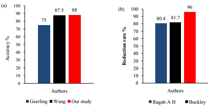
[29]	J. Geerling, D. Kendoff and M. Citak, et al., Intraoperative 3D imaging in calcaneal fracture care-clinical implications and decision making, J. Trauma., 66 (2009), 768–773.
[30]	R. Kakwani and M. Siddique, Operative compared with nonoperative treatment of displaced intra-articular calcaneal fractures: A prospective, randomized, controlled multicenter trial, J. Bone. Joint. Surg. Am., 84 (2002), 1733–1744.
[31]	A. H. Ragab, I. M. Mubark and A. M. Nagi, et al., Treatment of subtalar calcanean fractures using trans-osseous limited lateral approach, Ortop. Traumatol. Rehabil., 16 (2014), 629–638.

This article has been cited by:

1.	Gunjan Jha, Anshul Jha, Eugene John, 2024, A High Accuracy CNN for Breast Cancer Detection Using Mammography Images, 979-8-3503-8717-9, 1196, 10.1109/MWSCAS60917.2024.10658807
2.	Detection of Brain Tumor using Medical Images: A Comparative Study of Machine Learning Algorithms – A Systematic Literature Review, 2024, 13, 2278-2540, 77, 10.51583/IJLTEMAS.2024.130907
3.	Xiangquan Liu, Xiaoming Huang, Weakly supervised salient object detection via bounding-box annotation and SAM model, 2024, 32, 2688-1594, 1624, 10.3934/era.2024074
4.	Dekai Qiu, Tianhao Guo, Shengqi Yu, Wei Liu, Lin Li, Zhizhong Sun, Hehuan Peng, Dong Hu, Classification of Apple Color and Deformity Using Machine Vision Combined with CNN, 2024, 14, 2077-0472, 978, 10.3390/agriculture14070978
5.	Yu Xue, Zhenman Zhang, Ferrante Neri, Similarity surrogate-assisted evolutionary neural architecture search with dual encoding strategy, 2024, 32, 2688-1594, 1017, 10.3934/era.2024050
6.	Xiaoping Zhao, Liwen Jiang, Adam Slowik, Zhenman Zhang, Yu Xue, Evolving blocks by segmentation for neural architecture search, 2024, 32, 2688-1594, 2016, 10.3934/era.2024092
7.	Katuri Rama Krishna, Mohammad Arbaaz, Surya Naga Chandra Dhanekula, Yagna Mithra Vallabhaneni, MODIFIED VGG16 FOR ACCURATE BRAIN TUMOR DETECTION IN MRI IMAGERY, 2024, 14, 2391-6761, 71, 10.35784/iapgos.6035
8.	Maad M. Mijwil, Smart architectures: computerized classification of brain tumors from MRI images utilizing deep learning approaches, 2024, 1573-7721, 10.1007/s11042-024-20349-x
9.	B Gunasundari, H Kezia, T Dharanika, Pydala Anusha, Dasineni Yogitha, Vemula Lakshmi Prashanthi, 2024, Enhanced deep learning model using transfer learning to segment and detect brain tumors, 979-8-3503-7024-9, 1, 10.1109/ICCCNT61001.2024.10723895
10.	Mary Jane C. Samonte, Andrei Bench Mallari, Prince Rayly K. Reyes, John Caleb T. Tan, 2024, Applying Data Science in Computer Vision: Detection of Malignant and Benign Cancer Tumors, 979-8-3503-8826-8, 13, 10.1109/BDEE63226.2024.00010
11.	Bianca Antonia Fabian, Cristian-Cosmin Vancea, 2024, Efficient Methods for Improving Brain Tumors Diagnosis in MRI Scans Using Deep Learning, 979-8-3315-3997-9, 1, 10.1109/ICCP63557.2024.10793036
12.	Tanjim Mahmud, Mohammad Tarek Aziz, Taohidur Rahman, Koushick Barua, Anik Barua, Nanziba Basnin, Israt Ara, Nahed Sharmen, Mohammad Shahadat Hossain, Karl Andersson, 2024, Chapter 5, 978-3-031-73323-9, 39, 10.1007/978-3-031-73324-6_5
13.	Kingshuk Das Bakshi, S. Rani, S. Thanga Ramya, A. Bhagyalakshmi, Earli Manemma, Sumit Kushwaha, Identifying Neurological Disorders using Deep Learning with Biomedical Imaging Techniques, 2025, 1556-5068, 10.2139/ssrn.5109614
14.	R Rekha Sharmily, B Karthik, T Vijayan, 2024, MRI Brain Tumor Medical Images Multi Classification Using Deep Neural Networks, 979-8-3315-1859-2, 1, 10.1109/DELCON64804.2024.10866052
15.	Venkata Kiranmai Kollipara, Surendra Reddy Vinta, 2025, Chapter 43, 978-981-97-7177-6, 507, 10.1007/978-981-97-7178-3_43
16.	Huimin Qu, Haiyan Xie, Qianying Wang, Multi-convolutional neural network brain image denoising study based on feature distillation learning and dense residual attention, 2025, 33, 2688-1594, 1231, 10.3934/era.2025055
17.	Mehak Sharma, Krish Monga, Ripandeep Kaur, Sahil Bhardwaj, 2024, DEEPTUMORNET: BRAIN TUMOR CLASSIFICATION IN MEDICAL IMAGING, 979-8-3315-1905-6, 500, 10.1109/ICACCTech65084.2024.00087
18.	Madona B Sahaai, K Karthika, Aaron Kevin Cameron Theoderaj, EC-HDLNet: Extended coati-based hybrid deep dilated convolutional learning network for brain tumor classification, 2025, 107, 17468094, 107865, 10.1016/j.bspc.2025.107865
19.	Mohammed Nazneen Fathima, Prabhjot Singh, Simrandeep Singh, 2025, VTAF-Ensemble: A Hybrid Vision Transformer and Attention-based Learning Approach for Enhanced Brain Tumor Detection and Classification, 979-8-3315-2924-6, 1, 10.1109/ICISCN64258.2025.10934306
20.	Ankush Goyal, Yajnaseni Dash, Sudhir C. Sarangi, Ajith Abraham, 2025, Chapter 56, 978-3-031-81079-4, 589, 10.1007/978-3-031-81080-0_56
21.	S. Veluchamy, R. Bhuvaneswari, K. Ashwini, Samah Alshathri, Walid El-Shafai, HY-Deepnet : A new Optimal Deep transfer learning empowered framework for an autonomous Alzheimer’s disease detection and diagnosis system, 2025, 68, 22150986, 102058, 10.1016/j.jestch.2025.102058

Reader Comments

Your name:*

Email:*
© 2019 the Author(s), licensee AIMS Press. This is an open access article distributed under the terms of the Creative Commons Attribution License (http://creativecommons.org/licenses/by/4.0)