


Figure 1.
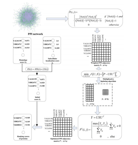
Overall workflow of IEPMSF for identifying essential proteins.
Citation: Nora Tilly, Daniel Kelterbaum. Investigating the Surface and Subsurface in Karstic Regions – Terrestrial Laser Scanning versus Low-Altitude Airborne Imaging and the Combination with Geophysical Prospecting[J]. AIMS Geosciences, 2017, 3(3): 352-374. doi: 10.3934/geosci.2017.3.352
| [1] | Lei Chen, Ruyun Qu, Xintong Liu . Improved multi-label classifiers for predicting protein subcellular localization. Mathematical Biosciences and Engineering, 2024, 21(1): 214-236. doi: 10.3934/mbe.2024010 |
| [2] | Yongyin Han, Maolin Liu, Zhixiao Wang . Key protein identification by integrating protein complex information and multi-biological features. Mathematical Biosciences and Engineering, 2023, 20(10): 18191-18206. doi: 10.3934/mbe.2023808 |
| [3] | Linlu Song, Shangbo Ning, Jinxuan Hou, Yunjie Zhao . Performance of protein-ligand docking with CDK4/6 inhibitors: a case study. Mathematical Biosciences and Engineering, 2021, 18(1): 456-470. doi: 10.3934/mbe.2021025 |
| [4] | Yutong Man, Guangming Liu, Kuo Yang, Xuezhong Zhou . SNFM: A semi-supervised NMF algorithm for detecting biological functional modules. Mathematical Biosciences and Engineering, 2019, 16(4): 1933-1948. doi: 10.3934/mbe.2019094 |
| [5] | Haipeng Zhao, Baozhong Zhu, Tengsheng Jiang, Zhiming Cui, Hongjie Wu . Identification of DNA-protein binding residues through integration of Transformer encoder and Bi-directional Long Short-Term Memory. Mathematical Biosciences and Engineering, 2024, 21(1): 170-185. doi: 10.3934/mbe.2024008 |
| [6] | Madeleine Dawson, Carson Dudley, Sasamon Omoma, Hwai-Ray Tung, Maria-Veronica Ciocanel . Characterizing emerging features in cell dynamics using topological data analysis methods. Mathematical Biosciences and Engineering, 2023, 20(2): 3023-3046. doi: 10.3934/mbe.2023143 |
| [7] | Wenjun Xia, Jinzhi Lei . Formulation of the protein synthesis rate with sequence information. Mathematical Biosciences and Engineering, 2018, 15(2): 507-522. doi: 10.3934/mbe.2018023 |
| [8] | Jinmiao Song, Shengwei Tian, Long Yu, Qimeng Yang, Qiguo Dai, Yuanxu Wang, Weidong Wu, Xiaodong Duan . RLF-LPI: An ensemble learning framework using sequence information for predicting lncRNA-protein interaction based on AE-ResLSTM and fuzzy decision. Mathematical Biosciences and Engineering, 2022, 19(5): 4749-4764. doi: 10.3934/mbe.2022222 |
| [9] | Sathyanarayanan Gopalakrishnan, Swaminathan Venkatraman . Prediction of influential proteins and enzymes of certain diseases using a directed unimodular hypergraph. Mathematical Biosciences and Engineering, 2024, 21(1): 325-345. doi: 10.3934/mbe.2024015 |
| [10] | Shun Li, Lu Yuan, Yuming Ma, Yihui Liu . WG-ICRN: Protein 8-state secondary structure prediction based on Wasserstein generative adversarial networks and residual networks with Inception modules. Mathematical Biosciences and Engineering, 2023, 20(5): 7721-7737. doi: 10.3934/mbe.2023333 |
Essential proteins are required for organism life, and their absence results in the loss of functional modules of protein complexes, as well as the death of the organism [1]. Essential proteins identification aids in the understanding of cell growth control mechanisms, the discovery of disease-causing genes and possible therapeutic targets, and has crucial theoretical and practical implications for drug development and disease therapy. In biological experiments, essential proteins are mainly identified by gene culling, gene suppression, transposon mutation and other methods, which cost lot of time and difficult unfortunately. Essential protein identification using computational approaches becomes achievable as high-throughput data accumulates. This identification method means utilizing the available data to find the key features that affect the importance of proteins and to determine if it is important of biological functions based on these features. The most common measuring technique is based on the topological properties of the PPI network to obtain network topology features, like Degree Centrality (DC) [2], Information Centrality (IC) [3], Closeness Centrality (CC) [4] and Subgraph Centrality (SC) [5], Betweenness Centrality (BC) [6], sum of Edge Clustering Coefficient Centrality (NC) [7]. These methods are sensitive to network structure, so false positive noise and data missing will reduce the performance of prediction easily.
In addition to characteristics of network topological, the biological characteristics involved in essential proteins identification mainly include sequence features and functional features. Zhang and Li et al. combined features of profiles of gene expression with topological features of PPI network, and proposed CoEWC [8] and PeC [9] methods respectively. Zhao et al. [10] put forward an essential protein detection model named POEM which utilize the module features of essential proteins. A weighted network with high confidence is built based on the topological structure and intrinsic characters of network and information about expression of genes, and overlap of functional modules, that coupling nature is weak and cohesive nature is strong, are discovered. In the end, the weighted density of the module to which the protein belongs was used to determine scores. Zhang et al. [11] got a new model named FDP to employs the global and local topological properties of network and protein homology information, to combine the dynamic PPI network at different times. In 2021, Zhong et al. [12] introduced a novel measuring approach named JDC that binary gene expression data with a dynamic threshold and combines the Jaccard index of similarity and degree centrality.
The method based on multi-source data integration effectively improve the prediction's level of accuracy and robustness. The commonly used processing method is to build a highly reliable weighted PPI network through weighted summary and the features are different for different prediction methods. The processing method of simple superposition will obfuscate the complicated relationship that exists between the multi-source data and generate artificial noise. The parameter setting is also matter which will influence the practical application of the algorithm. Non-negative matrix tri-factorization (NMTF) [13] is mainly used to analyze data matrices with non-negative elements, disintegrate the input matrix into three non-negative factor matrices, and approximate the input matrix through low-rank non-negative representation. It has been widely used in many fields such as text mining [14], recommendation system [15,16] and biological data analysis [17,18].
In view of the advantages of NMTF in data analysis and integrate protein homology information and subcellular location information to improve the prediction performance of essential proteins, an approach of non-negative matrix symmetric tri-factorization (IEPMSF) is offered as an optimal method for solving the noise problems in identifying essential proteins. In order to avoid more noise caused by multi-source data integration, this paper only uses the topological features of the original protein interaction data to construct the protein weighted network. But this method is not optimal because of the existence of false negatives and false positives. To solve this problem, the traditional NMTF algorithm is optimized. The factorization process is regarded as the "soft clustering" process of proteins, to predict the potential protein-protein interactions by a non-negative matrix symmetric tri-factorization algorithm (NMSTF), thus forming the optimal protein weighted network. Finally, to achieve the goal of predicting essential proteins, the homology information and subcellular location information of proteins are combined to create an initial score for each protein, which is then used to score and order each protein in the optimized network using the restart random walk algorithm.
This paper builds an improved protein-weighted network using the protein-protein interaction network and the NMSTF algorithm to increase the accuracy of important protein identification, and integrates subcellular localization information with protein homology information to design an essential model to identify essential proteins, IEPMSF. The model consists of three modules: weighted network building module, weighted network optimization module, and proteins scoring and sorting module.
Through topological analysis of yeast networks, the researchers found that PPI networks have small-world and non-scale characteristic [19] and that essential proteins have a strong connection with the topological properties of proteins. The co-neighbor coefficient is commonly utilized in the functional recognition [20] of proteins in PPI networks, demonstrating that the more similar neighbors two proteins in a network have, the more likely they are to interact. To measure the degree of interaction between the two proteins, we use the co-neighbor coefficient to give the edge weights of the network of protein interaction.
A simple undirected graph G = (V, E) can be a model of a PPI network. Here, the nodes set V = {v1, v2, …} as proteins, the edges set E = {e1, e2, e3 …} is a representation for the interaction of two different proteins. Defining a weighted network is WG = (V, E, P), where P(i, j) indicating the likelihood of the interaction of the vi and vj proteins, can be computed using the equation below :
| P(i,j)={|Nei(i)∩Nei(j)|2(|Nei(i)|−1)∗(|Nei(j)|−1)if |Nei(i)|>1 and |Nei(j)|>10otherwise | (1) |
where Nei(i) and Nei(j) respectively represent collection of neighbor nodes of the vi and vj, |Nei(i)∩Nei(j)| represent the number of common neighbors. If there are not any common neighbor proteins between the vi and vj, then P(i, j) = 0. We are going to assume that the probability of the interaction, the co-neighbor coefficient between the proteins, is independent of each other, and it's going to be in the range of 0 to 1.
As previously stated, false positives and false negatives can be found in PPI networks derived from high-throughput biological research. In other words, there are still some uncertainties in the construction of weighted networks based on protein interactions. NMTF was proposed by Ding in 2006 [13], which is an effective tool applied to recommendation systems successfully. Therefore, we can exploit the potential new protein interactions based on the existing protein and protein interaction data by using NMTF technology.
The traditional NMTF is the decomposition of the correlation matrix Yn*n into three low-rank sub-matrices, F∈Rn∗k, S∈Rk∗k and G∈Rk∗n, by which to approximate the original input matrix, as follows:
| P≈Y=FSGT | (2) |
Where the parameter k represents the factorization level and reflects the total number of possible vectors in the column spaces and row spaces. After being weighted to the protein interaction network with co-neighbor coefficients, the association matrix of the network can be constructed to represent the connection relationship between proteins. The elements in the correlation matrix are the co-neighbor values for each edge. Due to the singularity of nodes in the protein interaction network and the resulting correlation matrix is a symmetry matrix, the simple utilization of the conventional NMTF technology is not reasonably explanatory. Hart [21] pointed out that essential proteins often gather together, and the criticality of proteins is related to protein complexes rather than dependent on a single protein, which indicates that essential proteins have modular properties. Specifically, given a non-negative input matrix P, factor matrix S can be seen as the cluster index [14] of the vertex. Based on this, this paper proposes an improved NMTF algorithm called a non-negative matrix symmetric three-factors decomposition to rewrite Eq (2) into the following form:
| P≈Y=USUT | (3) |
Among them, U∈Rn∗k can be seen as "soft" clustering labels of proteins, and S∈Rk∗k as a correlation matrix between protein modules, S = ST. Then we can design the loss objective function of Eq (3) as follows:
| D=minU≥0,S≥0J(U,S)=||P−USUT||F | (4) |
Where ‖⋅‖F refers to the Frobenius specification. We use the multiplication update iteration technique to derive the objective function on the basis of employing the auxiliary function because the object function is a joint nonconvex problem. According to the rules of Squared frobenius norm we can know ||X||2 = Tr(XTX), which can solve D as follows:
| D=Tr(PTP−2PTUSUT+USTUTUSUT) | (5) |
Solve partial differential equations for U and S factors in Eq (5) respectively:
| ∂D∂U=−4PUS+4USUTUS |
| ∂D∂S=−2UTPU+2UTUSUTU | (6) |
Followed as Karush-Kuhn Tucker (KKT) complementary condition, we can find a static point, the KKT condition for U and S. These rules can be written as follows:
| ∂D∂UikUik=0 | (7) |
By Eq (7), we can get:
| (USUTUS−PUS)ikUik=0 |
| Uik=Uik(PUS)ik(USUTUS)ik | (8) |
Similarly, the S can be calculated using the same procedure:
| Sik=Sik(UTPU)ik(UTUSUTU)ik | (9) |
These rules can be expressed in a matrix form:
| Uik←Uik(PUS)ik(USUTUS)ik |
| Sik←Sik(UTPU)ik(UTUSUTU)ik | (10) |
According to the above multiplication update iteration rules, the final U and S can be calculated, so as to obtain the optimal Y = USUT approximating the original input matrix.
After the above data processing, we construct an optimized network association matrix, and conduct the corresponding standardization processing as follows:
| P∗(i,j)={max(Yij,Yji)∑Nk=0Yik,∑Nk=0Yik≠00,else | (11) |
The cumulative sum of each row of i in the matrix P* is 0 or 1.
We give an initial score to every protein from protein interaction network given by direct homology information and sub-cell localization information to improve the accuracy of essential protein prediction.
Studies have shown that when a protein has more homologous proteins in a reference species, it is highly likely to be an essential protein. The direct homology score of protein node vi is calculated by the equation below:
| HS(i)=HP(i)max1≤j≤|V|HP(j) | (12) |
where HP(i) represent how many direct homologous proteins in the reference species collection SC node vi has, as follows:
| HP(i)=∑m∈SCTNi where TNi={1ifvi∈XSm0otherwise | (13) |
where the XSm represents a collection of proteins with direct homologous proteins and is a subset of V. For those proteins that possess homologous proteins in all reference species, their direct homology score of 1 is given. Instead, if a protein does not have a direct homologous protein in all reference species, it has a score of 0.
Previous research has revealed that the essential state of proteins is not simply linked to the biological properties of PPI networks, but also to their location in space. Therefore, making full use of subcellular localization information is important for essential proteins prediction. Studies have shown that essential proteins are found in higher concentrations in certain subcellular locations than non-essential, and evolve more conserved [22]. Let L(R) be the protein set appearing at subcellular location r, and the frequency of protein appearing at it is possible to calculate each subcellular location r, as shown below:
| OF(r)=|L(r)|maxk∈R|L(k)| | (14) |
Where |L(r)| represents the number of proteins present at subcellular location r, and R represents the set containing each subcellular location. For a protein vi, let C(i) be the set of subcellular sites in which it occurs, and the definition of subcellular localization score LS(i) is the score of the maximum frequency of its occurrence at all subcellular locations by using the following equation:
| LS(i)=maxr∈C(i)OF(r) | (15) |
Combined with the direct homology score and subcellular localization score obtained by Eqs (12) and (15), the initial value score, IS(i), which is possible to compute the vi of each protein in the protein interaction network, with following equation:
| HS(i)=HS(i)×LS(i) | (16) |
Based on the weighted network constructed previously and the initial score based on the multi-source biological information, the final score, FS(i), of a protein vi from network can be calculated as bellow:
| FS(i)=α∑j∈Nei(i)P∗(i,j)FS(j)+(1−α)IS(i) | (17) |
where, Nei(i) shows the set of neighbor nodes of vi.
As can be seen from Eq (17), a protein's final score may be thought of as a linear combination of its multi-source bioinformatics mark and its neighboring correlation mark. Among them, the percentage of these two scores are adjusted using parameter a. When a is equal to 0, the final protein score is only related to the multi-source biological information score, and when the value of a is 1, the score is only related to the common neighbor properties of a protein. However, the amount of protein in the network is numerous and they have great computational complexity. Therefore, we can rewrite Eq (17) into the form of a matrix vector:
| FS(i)=α∗P∗∗FS+(1−α)∗IS | (18) |
Finally, the Jacobi iterative method can be used to quantitatively solve the Eq (18):
| FSt=α∗P∗∗FSt−1+(1−α)∗IS | (19) |
The number of iterations is represented by t = (0, 1, 2, …).
The validity of the IEPMSF model was evaluated by using the basic data of essential protein. The dataset incorporates essential protein dataset, PPI network dataset, protein homology information dataset, and subcellular location dataset. The benchmark essential proteins involved in the datasets are 1199 essential proteins, mainly from databases of MIPS [23], SGD [24], DEG [25], and SGDP [26]. The DIP [27] database is used to get the PPI network data. Excluding repeated protein interactions and the protein itself interactions, there are 5093 proteins and 24,743 interactions in the collection. The subcellular location data was downloaded from the COMPARTMENTS [28] database, which integrates MGD [29], SGD [24], UniProtKB [30], WormBase [31] and FlyBase [32] databases and eventually obtains 3923 proteins with subcellular location information. The homologous protein data is gathered from the InParanoid database's 7th edition [33], which included pair-wise comparisons of entire genomes of 99 eukaryotes and 1 prokaryote.
To determine the significance of proteins in the protein interaction network, proteins are compared with results derived by the algorithm IEPMSF or other existing ways, DC [2], IC [3], CC [4], BC [5], SC [6], NC [7], PeC [9], CoEWC [8], POEM [10], FDP [11] and JDC [12] for example.
In IEPMSF, the ordering score of the proteins are different depending on the a. To study the impact of parameter a on the capability of IEPMSF method, we experimented with several values ranging from 0 to 1 to see how they affected the accuracy of essential proteins prediction of IEPMSF. Table 1 contains detailed experimental data. The range of essential candidates selected is from the top 100 to the top 600. The ratio of actually essential proteins predicted determines predictive accuracy.
| a | Top 100 | Top 200 | Top 300 | Top 400 | Top 500 | Top 600 |
| 0 | 78.00% | 77.00% | 73.70% | 72.30% | 67.00% | 63.00% |
| 0.1 | 97.00% | 84.50% | 78.00% | 74.00% | 68.40% | 64.50% |
| 0.2 | 92.00% | 85.50% | 79.70% | 74.50% | 69.80% | 65.30% |
| 0.3 | 89.00% | 86.00% | 78.30% | 72.80% | 69.20% | 64.80% |
| 0.4 | 87.00% | 83.00% | 76.00% | 71.80% | 68.60% | 65.00% |
| 0.5 | 87.00% | 78.00% | 74.00% | 70.00% | 67.20% | 64.30% |
| 0.6 | 86.00% | 77.00% | 71.30% | 69.00% | 64.80% | 63.00% |
| 0.7 | 85.00% | 75.00% | 69.00% | 66.80% | 63.80% | 60.00% |
| 0.8 | 82.00% | 74.00% | 67.30% | 64.50% | 62.00% | 59.20% |
| 0.9 | 83.00% | 75.00% | 65.30% | 62.80% | 59.60% | 57.30% |
| 1 | 81.00% | 71.00% | 64.70% | 59.80% | 55.80% | 53.20% |
 DownLoad:
CSV
DownLoad:
CSV
As shown in Table 1, it is shown that when a = 0, the predicted essential protein only considers the direct homology of the protein, while when a = 1, the predicted essential protein only considers the co-neighbor information. When a = 0 or a = 1, the IEPMSF performs worse than the values of 0 to 1. This means that combination of the direct homologues of proteins and their neighbours can predict the required proteins more accurately than if only one of these properties is considered. To compare with other algorithms, as a = 0.1, when the top 100 ranking proteins are chosen as essential protein candidates, the accuracy can reach 0.97, as shown in the experimental findings in Figure 2.

When essential protein candidates with higher scores at different ratios (top 100,200,300,400,500, and 600) are chosen, their highest values are 97% (a = 0.1), 86% (a = 0.3), 79.7% (a = 0.2), 74.5% (a = 0.2), 69.8% (a = 0.2) and 65.3% (a = 0.2) respectively. The maximum level of accuracy is centered at a = 0.2 as the number of candidate proteins grows. Therefore, we set a as 0.2 to carry out the following experiments.
The PR curve is applied to further validate the capability of the various approaches. Firstly, according to the final scores computed by each technique, proteins in the protein interaction network are sorted in descending order. The preceding K proteins are considered essential proteins (positive dataset), whereas the remaining proteins are considered non-essential proteins (negative dataset), where the threshold K ranges from 1 to 5093. As the K values be changed, to produce the PR curve, the corresponding precision and recall values for each approach are computed, as illustrated in Figure 3. The PR curves of IEPMSF are compared with PR curves of centrality algorithms (DC, IC, CC, BC, SC, and NC) and of multi-source information fusion methods (PeC, CoEWC, POEM, JDC, and FDP) in Figure 3(a) and (b) respectively. As seen in Figure 3, the PR curve of the IEPMSF has much higher value than that of other algorithms.

To further examine the prediction performance of IEPMSF and other approaches, we apply the jackknife method. Figure 4 depicts the experimental outcomes. The number of putative essential proteins ranked first by each approach is represented on X-axis and the real number of important proteins found is represented on Y-axis. Performance of each method is compared in the area below the center line. Figure 4(a) demonstrate the outcome of a comparison between DC, IC, CC, BC, SC, NC and IEPMSF. From Figure 4(a), we see that the IEPMSF prediction of essential proteins is significantly more accurate than that of NC. Figure 4(b) shows the comparison of IEPMSF and existing methods based on multi-source information fusion (PeC, CoEWC, POEM, JDC and FDP). According to all of the experimental data. the accuracy of IEPMSF in predicting essential proteins is greater than the other 11 approaches, according to all of the experimental data.

The essential proteins identifying is not only a prerequisite in comprehending organism survival, but it is also critical for the discovery of disease-causing genes and possible therapeutic targets. An essential proteins identification model IEPMSF was designed in this paper. In order to avoid more noise caused by multi-source data integration, to build the weighted network, the model only uses the common neighbor topology properties of the nodes in the network from original PPI data. Considering the issue of false positive and false negative PPI data caused by high-throughput trials, and the clustering function of NMTF, the weighted network was optimized using the non-negative matrix symmetric tri-factorization (NMSTF) technique to uncover probable protein-protein interactions. Finally, the starting score of each protein node was calculated using the subcellular location and homologous proteins information, and the restart random walk method was used to score and rank each protein in the network. Compared with the topological centrality method and the traditional multi-source information integration method, the experimental findings reveal that the suggested essential proteins prediction approach, IEPMSF, significantly improves the performance of essential proteins prediction. On the basis of the existing work, how to design a more effective method to construct a weighted network based on multi-source information integration is the future research direction of essential proteins identification. In long term, we will investigate including more biological data during the weighted network construction step, and try to apply the model to other species.
This project is partially funded by the National Natural Science Foundation of China (61772089, 62006030), Natural Science Foundation of Hunan Province (2020JJ4648), Major Scientific and Technological Projects for collaborative prevention and control of birth defects in Hunan Province (2019SK1010).
The authors declare no competing interests.
| [1] | Zepp H (2014) Geomorphologie. 6th ed. UTB, Stuttgart. |
| [2] | Tilly N, Kelterbaum D, Zeese R (2016) Geomorphological mapping with terrestrial laser scanning and uav-based imaging. Int Arch Photogramm, Remote Sens Spat Inf Sci–ISPRS Arch 41: 591-597. |
| [3] | Large ARG, Heritage GL (2009) Laser Scanning – Evolution of the Discipline. In: Heritage GL, and Large ARG, editors. Laser Scanning for the Environmental Sciences, Wiley-Blackwell, West Sussex, UK. 1-20. |
| [4] |
Buckley SJ, Howell JA, Enge HD, et al (2008) Terrestrial laser scanning in geology: data acquisition, processing and accuracy considerations. J Geol Soc 165: 625-638. doi: 10.1144/0016-76492007-100

|
| [5] |
Tarolli P (2014) High-resolution topography for understanding Earth surface processes: Opportunities and challenges. Geomorphol 216: 295-312. doi: 10.1016/j.geomorph.2014.03.008
|
| [6] | Schaefer M, Inkpen R (2010) Towards a protocol for laser scanning of rock surfaces. Earth Surf Processes Landforms 35: 417-423. |
| [7] |
Colomina I, Molina P (2014) Unmanned aerial systems for photogrammetry and remote sensing: A review. ISPRS J Photogramm Remote Sens 92: 79-97. doi: 10.1016/j.isprsjprs.2014.02.013
|
| [8] |
Shahbazi M, Sohn G, Théau J, et al. (2015) Development and Evaluation of a UAV-Photogrammetry System for Precise 3D Environmental Modeling. Sensors 15: 27493-27524. doi: 10.3390/s151127493
|
| [9] |
Turner D, Lucieer A, Watson C (2012) An automated technique for generating georectified mosaics from ultra-high resolution Unmanned Aerial Vehicle (UAV) imagery, based on Structure from Motion (SFM) point clouds. Remote Sens 4: 1392-1410. doi: 10.3390/rs4051392
|
| [10] |
Westoby MJ, Brasington J, Glasser NF, et al. (2012) Structure-from-Motion photogrammetry: A low-cost, effective tool for geoscience applications. Geomorphol 179: 300-314. doi: 10.1016/j.geomorph.2012.08.021
|
| [11] |
Tong X, Liu X, Chen P, et al. (2015) Integration of UAV-Based Photogrammetry and Terrestrial Laser Scanning for the Three-Dimensional Mapping and Monitoring of Open-Pit Mine Areas. Remote Sens 7: 6635-6662. doi: 10.3390/rs70606635
|
| [12] | Smith MW, Carrivick JL, Quincey DJ (2015) Structure from motion photogrammetry in physical geography. Prog Phys Geogr 1-29. |
| [13] |
Ouédraogo MM, Degré A, Debouche C, et al. (2014) The evaluation of unmanned aerial system-based photogrammetry and terrestrial laser scanning to generate DEMs of agricultural watersheds. Geomorphol 214: 339-355. doi: 10.1016/j.geomorph.2014.02.016
|
| [14] | Butler DK (2005) Near-Surface Geophysics. Society of Exploration Geophysicists. https://doi.org/http://dx.doi.org/10.1190/1.9781560801719. |
| [15] |
Kidanu ST, Torgashov EV, Varnavina AV, et al. (2016) ERT-based Investigation of a Sinkhole in Greene County, Missouri. AIMS Geosci 2: 99-115. doi: 10.3934/geosci.2016.2.99
|
| [16] | Berglund JL, Mickus K, Gouzie D (2014) Determining a relationship between a newly forming sinkhole and a former dry stream using electric resistivity tomography and very low-frequency electromagnetics in an urban karst setting. Interpret 2: 17-27. |
| [17] | Siart C, Hecht S, Holzhauer I, et al. (2010) Karst depressions as geoarchaeological archives: The palaeoenvironmental reconstruction of Zominthos (Central Crete), based on geophysical prospection, sedimentological investigations and GIS. QuatInt 216: 75-92. |
| [18] |
Siart C, Ghilardi M, Forbriger M, et al. (2012) Terrestrial laser scanning and electrical resistivity tomography as combined tools for the geoarchaeological study of the Kritsa-Latô dolines (Mirambello, Crete, Greece). Géomorphol: Relief, Process, Environ 18: 59-74. doi: 10.4000/geomorphologie.9743
|
| [19] |
Siart C, Forbriger M, Nowaczinski E, et al. (2013) Fusion of multi-resolution surface (terrestrial laser scanning) and subsurface geodata (ERT, SRT) for karst landform investigation and geomorphometric quantification. Earth Surf Processes Landforms 38: 1135-1147. doi: 10.1002/esp.3394
|
| [20] |
Vlahovic T, Munda B (2012) Karst aquifers on small islands-the island of Olib, Croatia. Environ Monit Assess 184: 6211-6228. doi: 10.1007/s10661-011-2414-y
|
| [21] | Ahnert F (2009) Einführung in die Geomorphologie. 4th ed. UTB, Stuttgart. |
| [22] | Regierungspräsidium Freiburg (2017) Steckbrief Geotope–Ottensee NE von Mulfingen. Available from: http://www4.lgrb.uni-freiburg.de/serverbase/umn/etc/resources/link/gtk/gtk_1812.pdf. |
| [23] | Topcon Positioning Systems I (2006) HiPer Pro Operator's Manual. Available from: http://www.top-survey.com/top-survey/downloads/HiPerPro_om.pdf. |
| [24] | Riegl LMS GmbH (2010) Datasheet Riegl LMS-Z420i. Available from: http://www.riegl.com/uploads/tx_pxpriegldownloads/10_DataSheet_Z420i_03-05-2010.pdf. |
| [25] | DJI (2016) Datasheet Phantom 3. Available from: http://www.dji.com/de/product/phantom-3-adv. |
| [26] | DJI (2017) DJI GO app. Available from: http://www.dji.com/goapp. |
| [27] | GEO LOG (2017) Multi electrode system GeoTomMK8E1000 RES/IP/SP. Available from: http://geolog2000.de/EN/Geoelektrik/index.htm. |
| [28] |
Stummer P, Maurer H, Green AG (2004) Experimental design: Electrical resistivity data sets that provide optimum subsurface information. Geophys 69: 120-139. doi: 10.1190/1.1649381
|
| [29] |
Samouëlian A, Cousin I, Tabbagh A, et al. (2005) Electrical resistivity survey in soil science: A review. Soil Tillage Res 83: 173-193. doi: 10.1016/j.still.2004.10.004
|
| [30] |
Smith RC, Sjogren DB (2006) An evaluation of electrical resistivity imaging (ERI) in quaternary sediments, Southern Alberta, Canada. Geosph 2: 287-298. doi: 10.1130/GES00048.1
|
| [31] |
Winters G, Ryvkin I, Rudkov T, et al. (2015) Mapping underground layers in the super arid Gidron Wadi using electrical resistivity tomography (ERT). J Arid Environ Elsevier Ltd 121: 79-83. doi: 10.1016/j.jaridenv.2015.05.008
|
| [32] | Johnston K, Ver Hoef JM, Krivoruchko K, et al. (2001) Using ArcGIS Geostatistical Analyst. ESRI, USA. |
| [33] | Geotomo (2017) RES2DINVx64. Available from: http://www.geotomosoft.com. |
| [34] |
Loke MH, Barker RD (1996) Rapid least-squares inversion of apparent reistivity pseudosections by a quasi-Newton method. Geophys Prospect 44: 131-152. doi: 10.1111/j.1365-2478.1996.tb00142.x
|
| [35] |
Eltner A, Baumgart P (2015) Accuracy constraints of terrestrial Lidar data for soil erosion measurement: Application to a Mediterranean field plot. Geomorphol 245: 243-254. doi: 10.1016/j.geomorph.2015.06.008
|
| [36] |
Favalli M, Fornaciai A, Isola I, et al. (2012) Multiview 3D reconstruction in geosciences. Comput Geosci 44: 168-176. doi: 10.1016/j.cageo.2011.09.012
|
| [37] | Riegl LMS GmbH (2015) Datasheet Riegl VZ-2000. Available from: http://www.riegl.com/uploads/tx_pxpriegldownloads/DataSheet_VZ-2000_2015-03-24.pdf. |
| [38] | Leica Geoystems (2015) Datasheet Leica ScanStation P40. Available from: http://www.leica-geosystems.com/downloads123/hds/hds/general/brochures-datasheet/Leica_ScanStation_P30-P40_Plant_DS_en.pdf. |
| [39] | Velodyne (2014) Velodyne HDL-64E User's Manual. Available from: http://www.velodynelidar.com/lidar/products/manual/63-HDL64E S2 Manual_Rev D_2011_web.pdf. |
| [40] | Liang X, Kukko A, Kaartinen H, et al. (2013) Possibilities of a personal laser scanning system for forest mapping and ecosystem services. Sens 14: 1228-1248. |
| [41] |
Ryding J, Williams E, Smith M, et al. (2015) Assessing Handheld Mobile Laser Scanners for Forest Surveys. Remote Sens 7: 1095-1111. doi: 10.3390/rs70101095
|
| [42] |
Bates KT, Rarity F, Manning PL, et al. (2008) High-resolution LiDAR and photogrammetric survey of the Fumanya dinosaur tracksites (Catalonia): implications for the conservation and interpretation of geological heritage sites. J Geol Soc 165: 115-127. doi: 10.1144/0016-76492007-033
|
| [43] | Nex F, Rinaudo F (2011) LiDAR or Photogrammetry? Integration is the answer. Italian J Remote Sens 43: 107-121. |
| [44] |
Fabris M, Baldi P, Anzidei M, et al. (2010) High resolution topographic model of Panarea Island by fusion of photogrammetric, lidar and bathymetric digital terrain models. Photogramm Rec 25: 382-401. doi: 10.1111/j.1477-9730.2010.00600.x
|
| [45] |
Ahmed S, Carpenter PJ (2003) Geophysical response of filled sinkholes, soil pipes and associated bedrock fractures in thinly mantled karst, east-central Illinois. Environ Geol 44: 705-716. doi: 10.1007/s00254-003-0812-3
|
| [46] |
Mauriello P, Monna D, Patella D (1998) 3D geoelectric tomography and archaeological applications. Geophys Prospect 46: 543-570. doi: 10.1046/j.1365-2478.1998.00102.x
|
| [47] |
Alaia R, Patella D, Mauriello P (2008) Application of geoelectrical 3D probability tomography in a test-site of the archaeological park of Pompei (Naples, Italy). J Geophys Eng 5: 67-76. doi: 10.1088/1742-2132/5/1/007
|
| 1. | Yane Li, Chengfeng Wang, Haibo Gu, Hailin Feng, Yaoping Ruan, ESMDNN-PPI: a new protein–protein interaction prediction model developed with protein language model of ESM2 and deep neural network, 2024, 35, 0957-0233, 125701, 10.1088/1361-6501/ad761c |
Figures(6) / Tables(1)

Nora Tilly, Daniel Kelterbaum. Investigating the Surface and Subsurface in Karstic Regions – Terrestrial Laser Scanning versus Low-Altitude Airborne Imaging and the Combination with Geophysical Prospecting[J]. AIMS Geosciences, 2017, 3(3): 352-374. doi: 10.3934/geosci.2017.3.352

| a | Top 100 | Top 200 | Top 300 | Top 400 | Top 500 | Top 600 |
| 0 | 78.00% | 77.00% | 73.70% | 72.30% | 67.00% | 63.00% |
| 0.1 | 97.00% | 84.50% | 78.00% | 74.00% | 68.40% | 64.50% |
| 0.2 | 92.00% | 85.50% | 79.70% | 74.50% | 69.80% | 65.30% |
| 0.3 | 89.00% | 86.00% | 78.30% | 72.80% | 69.20% | 64.80% |
| 0.4 | 87.00% | 83.00% | 76.00% | 71.80% | 68.60% | 65.00% |
| 0.5 | 87.00% | 78.00% | 74.00% | 70.00% | 67.20% | 64.30% |
| 0.6 | 86.00% | 77.00% | 71.30% | 69.00% | 64.80% | 63.00% |
| 0.7 | 85.00% | 75.00% | 69.00% | 66.80% | 63.80% | 60.00% |
| 0.8 | 82.00% | 74.00% | 67.30% | 64.50% | 62.00% | 59.20% |
| 0.9 | 83.00% | 75.00% | 65.30% | 62.80% | 59.60% | 57.30% |
| 1 | 81.00% | 71.00% | 64.70% | 59.80% | 55.80% | 53.20% |
DownLoad:
CSV
| a | Top 100 | Top 200 | Top 300 | Top 400 | Top 500 | Top 600 |
| 0 | 78.00% | 77.00% | 73.70% | 72.30% | 67.00% | 63.00% |
| 0.1 | 97.00% | 84.50% | 78.00% | 74.00% | 68.40% | 64.50% |
| 0.2 | 92.00% | 85.50% | 79.70% | 74.50% | 69.80% | 65.30% |
| 0.3 | 89.00% | 86.00% | 78.30% | 72.80% | 69.20% | 64.80% |
| 0.4 | 87.00% | 83.00% | 76.00% | 71.80% | 68.60% | 65.00% |
| 0.5 | 87.00% | 78.00% | 74.00% | 70.00% | 67.20% | 64.30% |
| 0.6 | 86.00% | 77.00% | 71.30% | 69.00% | 64.80% | 63.00% |
| 0.7 | 85.00% | 75.00% | 69.00% | 66.80% | 63.80% | 60.00% |
| 0.8 | 82.00% | 74.00% | 67.30% | 64.50% | 62.00% | 59.20% |
| 0.9 | 83.00% | 75.00% | 65.30% | 62.80% | 59.60% | 57.30% |
| 1 | 81.00% | 71.00% | 64.70% | 59.80% | 55.80% | 53.20% |
