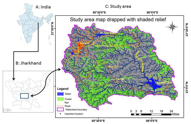
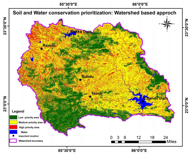
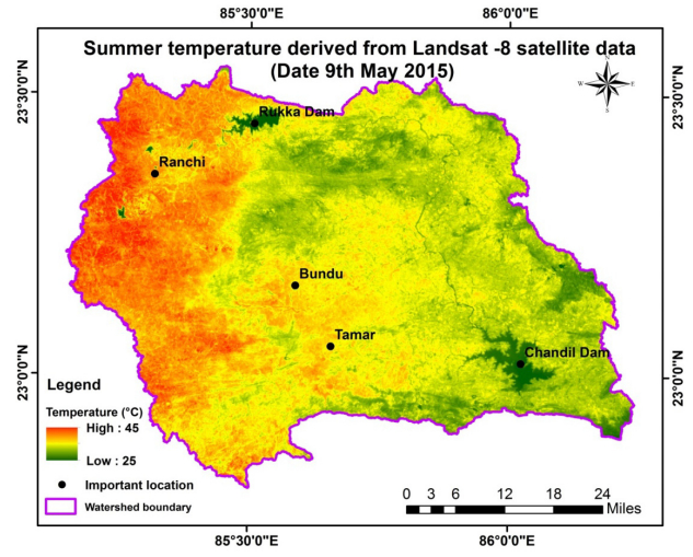
Citation: Firoz Ahmad, Laxmi Goparaju. Soil and Water Conservation Prioritization Using Geospatial Technology – a Case Study of Part of Subarnarekha Basin, Jharkhand, India[J]. AIMS Geosciences, 2017, 3(3): 375-395. doi: 10.3934/geosci.2017.3.375
| [1] | Zhun Han, Hal L. Smith . Bacteriophage-resistant and bacteriophage-sensitive bacteria in a chemostat. Mathematical Biosciences and Engineering, 2012, 9(4): 737-765. doi: 10.3934/mbe.2012.9.737 |
| [2] | Baojun Song, Wen Du, Jie Lou . Different types of backward bifurcations due to density-dependent treatments. Mathematical Biosciences and Engineering, 2013, 10(5&6): 1651-1668. doi: 10.3934/mbe.2013.10.1651 |
| [3] | Timothy C. Reluga, Jan Medlock . Resistance mechanisms matter in SIR models. Mathematical Biosciences and Engineering, 2007, 4(3): 553-563. doi: 10.3934/mbe.2007.4.553 |
| [4] | Linda J. S. Allen, P. van den Driessche . Stochastic epidemic models with a backward bifurcation. Mathematical Biosciences and Engineering, 2006, 3(3): 445-458. doi: 10.3934/mbe.2006.3.445 |
| [5] | Miller Cerón Gómez, Eduardo Ibarguen Mondragon, Eddy Lopez Molano, Arsenio Hidalgo-Troya, Maria A. Mármol-Martínez, Deisy Lorena Guerrero-Ceballos, Mario A. Pantoja, Camilo Paz-García, Jenny Gómez-Arrieta, Mariela Burbano-Rosero . Mathematical model of interaction Escherichia coli and Coliphages. Mathematical Biosciences and Engineering, 2023, 20(6): 9712-9727. doi: 10.3934/mbe.2023426 |
| [6] | Kento Okuwa, Hisashi Inaba, Toshikazu Kuniya . An age-structured epidemic model with boosting and waning of immune status. Mathematical Biosciences and Engineering, 2021, 18(5): 5707-5736. doi: 10.3934/mbe.2021289 |
| [7] | Lingli Zhou, Fengqing Fu, Yao Wang, Ling Yang . Interlocked feedback loops balance the adaptive immune response. Mathematical Biosciences and Engineering, 2022, 19(4): 4084-4100. doi: 10.3934/mbe.2022188 |
| [8] | Olga Vasilyeva, Tamer Oraby, Frithjof Lutscher . Aggregation and environmental transmission in chronic wasting disease. Mathematical Biosciences and Engineering, 2015, 12(1): 209-231. doi: 10.3934/mbe.2015.12.209 |
| [9] | Maoxing Liu, Yuming Chen . An SIRS model with differential susceptibility and infectivity on uncorrelated networks. Mathematical Biosciences and Engineering, 2015, 12(3): 415-429. doi: 10.3934/mbe.2015.12.415 |
| [10] | G. V. R. K. Vithanage, Hsiu-Chuan Wei, Sophia R-J Jang . Bistability in a model of tumor-immune system interactions with an oncolytic viral therapy. Mathematical Biosciences and Engineering, 2022, 19(2): 1559-1587. doi: 10.3934/mbe.2022072 |
Bacteriophage or virulent phage is a virus which can grow and replicate by infecting bacteria. Once residing in bacteria, phage grow quickly, which result in the infection of bacteria and drive the bacteria to die [17]. Thus, we can view them as bacteria predators and use them to cure the diseases induced by infecting bacteria [9,35]. Phage therapy has become a promising method because of the emergence of antibiotic resistant bacteria [12,9]. Indeed, as a treatment, phages have several advantages over antibiotics. Phages replicate and grow exponentially, while antibiotics are not [47]. Generally speaking, a kind of phages infect only particular classes of bacteria, and this limitation of their host is very beneficial to cure the diseases. Moreover, phages are non-toxic, and cannot infect human cells. Hence, there are fewer side effects as compared to antibiotics [12,35].
It is important to understand the interaction dynamics between bacteria and phage to design an optimal scheme of phage therapy. There have been a number of papers that study the mathematical models of bacteriophages (see, for example, [1,2,3,4,8,9,10,11,21,23,28,42] and the references cited therein). Campbell [11] proposed a deterministic mathematical model for bacteria and phage, which is a system of differential equations containing two state variables, susceptible bacteria
It was observed that phage can exert pressure on bacteria to make them produce resistance through loss or modification of the receptor molecule to which a phage binds with an inferior competition ability for nutrient uptake [25]. More recently, biological evidences are found that there exists an adaptive immune system across bacteria, which is the Clustered regularly interspaced short palindromic repeats (CRISPRs) along with Cas proteins [6,14,13,18,26,27,31,41]. In this system, phage infection is memorized via a short invader sequence, called a proto-spacer, and added into the CRISPR locus of the host genome. And, the CRISPR/Cas system admits heritable immunity [14,13,18,26,31]. The replication of infecting phage in bacteria is aborted if their DNA matches the crRNAs (CRISPR RNAs) which contains these proto-spacer. On the other hand, if there is no perfect pairing between the proto-spacer and the foreign DNA (as in the case of a phage mutant), the CRISPR/Cas system is counteracted and replication of the phage DNA can occur [19,34,33,39]. Therefore, the CRISPR/Cas system participates in a constant evolutionary battle between phage and bacteria [7,13,27,47].
Mathematical models are powerful in understanding the population dynamics of bacteria and phages. Han and Smith [23] formulated a mathematical model that includes a phage-resistant bacteria, where the resistant bacteria is an inferior competitor for nutrient. Their analytical results provide a set of sufficient conditions for the phage-resistant bacteria to persist. Recently, mathematical models have been proposed to study the contributions of adaptive immune response from CRISPR/Cas in bacteria and phage coevolution [27,29]. In these papers, numerical simulations are used to find how the immune response affects the coexistence of sensitive strain and resistance strain of bacteria. In the present paper, we extend the model in [23] by incorporating the CRISPR/Cas immunity on phage dynamics. Following [23], we focus on five state variables:
Let
| ˙R=D(R0−R)−f(R)(S+μM),˙S=−DS+f(R)S−kSP,˙M=−DM+μf(R)M+εkSP−k′MP,˙I=−DI+(1−ε)kSP+k′MP−δI,˙P=−DP−kSP−kMP+bδI, | (1) |
where a dot denotes the differentiation with respect to time
The paper is organized as follows. In the next section we present the mathematical analysis of the model that include the stability and bifurcation of equilibria. Numerical simulations are provided in Section
In this section, we present the mathematical analysis for the stability and bifurcations of equilibria of (1). We start with the positivity and boundedness of solutions.
Proposition 1. All solutions of model (1) with nonnegative initial values are nonnegative. In particular, a solution
Proof. We examine only the last conclusion of the proposition. First, we claim that
| S(t)=S(0)e∫t0[−D−kP(θ)+f(R(θ))]dθ>0. |
In a similar way we can show the positivity of
Proposition 2. All nonnegative solutions of model (1) are ultimately bounded.
Proof. Set
| L(t)=R(t)+S(t)+M(t)+I(t)+1bP(t). |
Calculating the derivative of
| ˙L(t)=DR0−DR(t)−DS(t)−DM(t)−DI(t)−1bDP(t) −1bkS(t)P(t)−1bkM(t)P(t)≤DR0−DL(t). |
It follows that the nonnegative solutions of
| lim supt→∞L(t)≤R0. | (2) |
Therefore, the nonnegative solutions of model (1) are ultimately bounded.
| m>D,f(R0)>D. | (3) |
Then
| μm>D,μf(R0)>D. | (4) |
It is easy to see that (3) and (4) imply
| λ1<μλ2<λ2. |
Thus, the competitive exclusion in the absence of phage infection holds [24], and the boundary equilibrium
The basic reproduction number
| F=(0(1−ε)k(R0−λ1)00), |
and
| V=(D+δ0−bδD+k(R0−λ1)), |
and is defined as the spectral radius of
| R0=√bδ(1−ε)k(R0−λ1)(D+δ)[D+k(R0−λ1)]. |
Analogously, the basic reproduction number
| RM0=√bδκ(R0−λ2)(D+δ)[D+k(R0−λ2)]. |
Theorem 2.1. The infection-free equilibrium
The proof of Theorem 2.1 is postponed to Appendix.
Theorem 2.2. The infection-free equilibrium
Proof. Define a Lyapunov function by
| V(t)=R(t)−R1−∫RR1f(R1)f(ξ)dξ+S(t)−S1−S1lnSS1+M(t)+I(t)+1bP(t), |
where
| ˙V(t)=(1−f(R1)f(R))˙R(t)+(1−S1S)˙S(t)+˙M(t)+˙I(t)+1b˙P(t)=D(R0−R)−D(R0−R)f(R1)f(R)+(S+μM)f(R1)+(D+kP−f(R))S1−DS−DM−DI−DbP−kSP+kMPb=D(R0−R1)(2−f(R1)f(R)−f(R)f(R1))−D(R−R1)(1−f(R1)f(R))−D(1−μ)M−DI+(kS1−Db)P−kSP+kMPb. |
Since
| D0={(R,S,M,I,P)∣˙V=0}. |
It is easy to examine that the largest invariant set in
| {(R,S,M,I,P)∣R=λ1,S=S1,M=0,I=0,P=0}. |
It follow from the LaSalle's invariance principle [22] that
In this subsection, we consider the infection equilibria of system (1) which satisfy
| D(R0−R)−f(R)S−μf(R)M=0,−DS+f(R)S−kSP=0,−DM+μf(R)M+εkSP−k′MP=0,−DI+(1−ε)kSP+k′MP−δI=0,−DP−kSP−kMP+bδI=0. | (5) |
If
| D(R0−R3)−μf(R3)M3=0,−DM3+μf(R3)M3−k′M3P3=0,−DI3+k′M3P3−δI3=0,−DP3−kM3P3+bδI3=0. |
It follows that
| P3=μf(R3)−Dk′,M3=D(R0−R3)μf(R3),I3=k′M3P3D+δ, |
and
| −DP3−kM3P3+bδI3=P3(kA2M3−D)=0, |
where
| g(R3):=R23+(a+mA−R0)R3−R0a=0, | (6) |
where
| A=μkD+δbδκ−(D+δ). |
By direct calculations, we obtain
| g(R0)=mAR0>0,g(λ2)=(λ2−R0)(λ2+a)+mAλ2. |
Since
| A<(R0−λ2)(λ2+a)mλ2=μ(R0−λ2)D, |
which is equivalent to
Theorem 2.3. The infection equilibrium
To study the local stability of infection equilibria
| a1=kM3+3D+δ+μM3f′(R3),a2=kM3(μM3f′(R3)+2D−μf(R3))+D(2D+δ)+(2D+δ+μf(R3))μM3f′(R3),a3=DkM3(μM3f′(R3)+D−μf(R3))+D(D+δ)(μf(R3)−D)+μf(R3)μM3f′(R3)(2D+δ),a4=kA2(D+δ)(μM3f′(R3)+D)(μf(R3)−D). | (7) |
Moreover, for
| λ3=f−1(D(1−κ)/(μ−κ)). | (8) |
Theorem 2.4. The infection-resistant equilibrium
| κ<μ,R3>λ3,a1a2>a3,(a1a2−a3)a3−a4a21>0, | (9) |
and is unstable when
| κ<μ,R3<λ3,a1a2>a3,(a1a2−a3)a3−a4a21>0. | (10) |
The proof of Theorem 2.4 is given in Appendix.
Let us now consider the existence of coexistence equilibrium of (1). Denote such an equilibrium by
| P4=f(R4)−Dk,M4=εD(R0−R4)(f(R4)−D)[D−μf(R4)+με(f(R4)−D)+k′P4]f(R4),S4=D(R0−R4)[k′P4+D−μf(R4)][D−μf(R4)+με(f(R4)−D)+k′P4]f(R4),I4=[(1−ε)kS4+k′M4]P4D+δ. | (11) |
Since
| f(R4)>D,k′P4+D−μf(R4)>0. | (12) |
Note that
| F(R4):=k′P4+D−μf(R4)=D(1−κ)+(κ−μ)f(R4), |
where
Note that
| −D+(bδκD+δ−1)kM4+(bδ1−εD+δ−1)kS4=0. | (13) |
Set
| A1=bδ(1−ε)/(D+δ)−1,A2=bδκ/(D+δ)−1. | (14) |
Using (11) and
| G(R4):=k(R0−R4)(e1+e2Df(R4))−(e3f(R4)+e4)=0, |
where
| e1=κA1−μA1+εA2,e2=A1−κA1−εA2,e3=με−μ+κ,e4=(1−με−κ)D. |
Let
Evidently,
| G(λ2)=−D+kA2(R0−λ2)=(D+k(R0−λ2))(RM−1). |
Thus,
| G(λ1)=−D+kA1(R0−λ1)=(D+k(R0−λ1))(R20−1). |
Hence,
For the case where
| G(λ3)=D(R0−λ3)(e1+e2Df(λ3))−(e3f(λ3)+e4)=D(R0−λ3)εA2(1−μ)1−κ−μεD(1−μ)μ−κ. |
Since
| λ3≥R0−μ(1−κ)A2(μ−κ), | (15) |
and
| λ3<R0−μ(1−κ)A2(μ−κ). | (16) |
Solve
| b∗=D+δδ((μ−κ)(R0−λ3)(1−κ)μ+1). |
Notice that
| P4=f(λ3)−Dk=D(1−κ)k(μ−κ),M4=D(R0−λ3)(f(λ3)−D)μf(λ3),I4=k′M4P4D+δ. |
Set
| R∗:=R0RM0=√(D+k(R0−λ2))(1−ε)(R0−λ1)κ(R0−λ2)(D+k(R0−λ1)). |
Solving
| ε=ε∗:=1−κ(R0−λ2)(D+k(R0−λ1))(D+k(R0−λ2))(R0−λ1). |
Thus,
Let us consider three cases:
The following Theorem states the existence of infection equilibria of (1) according to the above discussions.
Theorem 2.5. Let
For
Proof. Note that
This theorem indicates that the system (1) exhibits a backward bifurcation as
Notice that the equilibrium
Theorem 2.6. Let
For
For
The proof of this Theorem is omitted because it is similar to it for Theorem 2.5.
Theorem 2.6 presents the conditions for a forward bifurcation of the infection-free equilibrium and a transcritical bifurcation of the coexist equilibrium. Note that for
We now explore the persistence and extinction of phages in the case where
Theorem 2.7. Let
(
| limt→∞(R(t),S(t),M(t),I(t),P(t))=(λ1,R0−λ1,0,0,0) |
if
(
| lim inft→∞S(t)>η,lim inft→∞M(t)>η,lim inft→∞I(t)>η,lim inft→∞P(t)>η. |
Proof.
| f∞=lim supt→∞f(t),f∞=lim inft→∞f(t). |
First, we claim that a positive solution of (1) admits
| ˙S≤−DS+f(R)S≤−DS+f(R0+η0−S)S,for all large t, |
where
| ˙I≤−DI+(1−ε)k(R0−λ1+η1)P−δI,˙P≤−DP−k(R0−λ1−η1)P+bδI, | (17) |
where
| ˙I=−DI+(1−ε)k(R0−λ1+η1)P−δI,˙P=−DP−k(R0−λ1−η1)P+bδI. | (18) |
The Jacobian matrix of (18) is
| J1:=(−(D+δ)(1−ε)k(R0−λ1+η1)bδ−(D+k(R0−λ1−η1)). |
Since
| ˙R=D(R0−R)−f(R)(S+μM),˙S=−DS+f(R)S,˙M=−DM+μf(R)M. | (19) |
Since
| X={(R,S,M,I,P):R≥0,S≥0,M≥0,I≥0,P≥0},X0={(R,S,M,I,P)∈X:I>0,P>0},∂X0=X∖X0. |
We wish to show that (1) is uniformly persistent with respect to
By Proposition 1, we see that both
| J∂={(R,S,M,I,P)∈X:I=0,P=0}. |
It is clear that there are three equilibria
Note that (3) and (4) imply that a positive solution of (1) cannot approach
| ˙I≥−DI+(1−ε)k(R0−λ1−η2)P−δI,˙P≥−DP−k(R0−λ1+η2)P+bδI, | (20) |
where
| J2:=(−(D+δ)(1−ε)k(R0−λ1−η2)bδ−(D+k(R0−λ1+η2)). |
Since
| ˙I=−DI+(1−ε)k(R0−λ1−η2)P−δI,˙P=−DP−k(R0−λ1+η2)P+bδI | (21) |
tend to infinity as
By adopting the same techniques as above, we can show that the population
| ˙M≥−DM+εkSP. |
This, together with the uniform persistence of population
In this section, we implement numerical simulations to illustrate the theoretical results and explore more interesting solution patterns of model (1). Take the same parameter values as those in [23] where
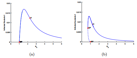 Figure 1. Bifurcation graphs for
 To demonstrate the second case where
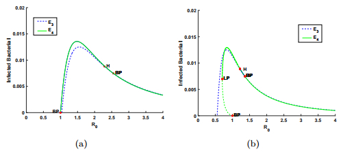 Figure 2. Bifurcation graphs for case
 To show the case
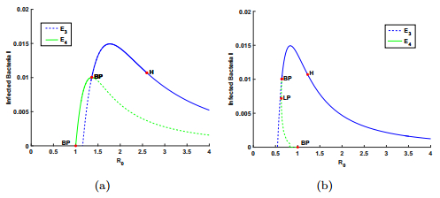 Figure 3. Bifurcation graphs for case
 With the help of
As discussed above, a bistable coexistence between the infection-free equilibrium and an infection equilibrium may occur when
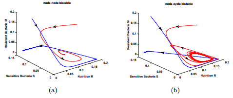 Figure 4. Graphs of bistable behaviors in case
 In this paper, we have developed a bacteriophage mathematical model based on CRISPR/Cas immune system. By combining theoretical analysis and numerical simulations, we have found that the model exhibits some new dynamical behaviors than the model without the immune responses in [23]. More specifically, the introduction of the CRISPR/Cas immune system induces a backward bifurcation from the infection-free equilibrium or a transcritical bifurcation from the coexist equilibrium, which means that although the basic infection reproduction number is below unity, the phage could coexist with bacteria. The coexistence of a stable infection-free equilibrium with a stable infection equilibrium(or stable coexist equilibrium), the bistable phenomenon of a stable infection-free equilibrium and a stable periodic solution are found, which are shown in panel (a) of Fig. 4 and panel (b) of Fig. 4. They provide reasonable explanations for the complexity of phage therapy [9,29] or bacteria-phages coevolution [13], and the coexistence of bacteria with phage in the biological experiments [20,29]. In contrast, there is no the backward bifurcation or bistable phenomena in the models of previous studies [23,42] where the immune response is ignored.
For case
The mathematical analysis for the stability and bifurcation of equilibria of (1) in this paper present some insights into the underlying phage infection mechanisms by considering the CRISPR/Cas system in bacteria. It will be interesting to consider the analytical conditions for the Hopf bifurcation and the homoclinic bifurcation of the model and reveal how the immune response affect these bifurcations. It will be also interesting to consider the effect of latent period of infection like it in [23] or the nonlinear death rates like those in [29]. We leave these as future researches.
We are very grateful to the anonymous referees for careful reading and valuable comments which have led to important improvements of our original manuscript.
Proof Theorem 2.1. Let
| J(E1)=(−D−S1f′(λ1)−D−μD00S1f′(λ1)000−kS100−D+μD0εkS1000−D−δ(1−ε)kS1000bδ−D−kS1), |
where
| (ω+D)(ω+S1f′(λ1))[ω2+(2D+δ+kS1)ω+f0](ω+D(1−μ))=0, |
where
| f0=(D+kS1)(D+δ)(1−R20). |
Since
Proof Theorem 2.4. Evaluating the Jacobian of (1) at
| J(E3)=(−D−μM3f′(R3)−f(R3)−μf(R3)000−D+f(R3)−kP3000μM3f′(R3)εkP300−k′M30(1−ε)kP3k′P3−D−δk′M30−kP3−kP3bδ−D−kM3). |
Using
| (ω−f(R3)+kP3+D)(ω4+a1ω3+a2ω2+a3ω+a4)=0, |
where
| F1(ω)=ω−f(R3)+kP3+D,F2(ω)=ω4+a1ω3+a2ω2+a3ω+a4. |
Note that
| f(R3)−kP3−D=(1−μκ)f(R3)+(1κ−1)D:=F0(ω). |
It is easy to see
| f(R3)>D(1−κ)μ−κ, |
which is equivalent to
| [1] | Kinthada NR, Gurram MK, Eadara A, et al. (2014) Land Use/land cover and NDVI Analysis for monitoring the health of micro-watersheds of Sarada River Basin, Visakhapatnam District, India. J Geol Geosci 3: 2. |
| [2] |
Walling DE (2006) Human impact on land-ocean sediment transfer by the world's rivers. Geomorphol 79: 192-216. doi: 10.1016/j.geomorph.2006.06.019

|
| [3] |
Wang HJ, Saito Y, Zhang Y, et al. (2011) Recent changes of sediment flux to the western Pacific Ocean from major rivers in East and Southeast Asia. Earth-Sci Rev 108: 80-100. doi: 10.1016/j.earscirev.2011.06.003
|
| [4] |
Phillips-Howard KD, Lyon F (1994) Agricultural intensification and the threat to soil fertility in Africa: evidence from the Jos Plateau, Nigeria. Geogr J 160: 252-265. doi: 10.2307/3059608
|
| [5] | Fairhead J, Leach M (1996) Misreading the African landscape: society and ecology in a forest-savanna mosaic. African Studies Series, 90. Cambridge University Press. |
| [6] | Reij C, Scoones I, Toulmin C, et al. (1996) Sustaining the soil: indigenous soil and water conservation in Africa. Earthscan Publications, London. |
| [7] | Mortimore M, Harris FMA, Turner B (1999) Implications of land use change for the production of plant biomass in densely populated Sahelo-Sudanian shrub-grasslands in north-east Nigeria. GlobEcol Biogeogr 8: 243-256. |
| [8] | Tullos DD, Neumann M (2006) A qualitative model for analyszing the effects of anthropogenic activities in the watershed on benthic macro invertebrate communities. |
| [9] |
Sabahattin I, Emrah D, Latif K, et al. (2008) Effects of anthropogenic activities on the lower Sakarya River. Catena 75: 172-181. doi: 10.1016/j.catena.2008.06.001
|
| [10] | Panhalkar SS, Mali SP, Pawar CT (2012) Morphometric Analysis and Watershed Development Prioritization of Hiranykeshi Basin in Maharashtra, India. Int J Environ Sci 3: 525-534. |
| [11] |
Biard F, Baret F (1997) Crop Residue Estimation Using Multiband Reflectance. Remote Sens Environ 59: 530-536. doi: 10.1016/S0034-4257(96)00125-3
|
| [12] | Gajbhiye S, Mishra S, Pandey A (2013) Prioritizing erosion prone area through morphometric analysis: an Remote sensing and GIS perspective. Appl Water Sci 4: 51-61. |
| [13] | Rao M, Hines K, Obreza T, et al. (2015) Watersheds of Florida: Understanding a watershed approach to water management. Soil Water Sci. |
| [14] | Gupta P, Uniyal S (2013) Watershed Prioritization of Himalayan Terrain Using SYI model. Int J Adv Remote Sens, GIS and Geogr 1: 42-48 |
| [15] | Tideman EM (1996) Watershed Management: Guidelines for Indian Conditions. J Chromatogr A 1154: 342. |
| [16] |
Ndulue EL, Mbajiorgu CC, Ugwu SN, et al. (2015). Assessment of land use/cover impacts on runoff and sediment yield using hydrologic models: A review. J Ecol Nat Environ 7: 46-55. doi: 10.5897/JENE2014.0482
|
| [17] | Khan S, Bhuvaneshwari B, Qureshi M (1999) Land use/Land covers mapping and change detection using remote sensing and GIS: a case study of Jamuna and its Environs. Socio-Econ Dev Rec 6: 32-33. |
| [18] | Sreenivasulu V, UdayaBhaskar P (2010) Change Detection in Land use and Land cover Using Remote Sensing and GIS Techniques. Int J Eng Sci Technol 2: 7758-7762. |
| [19] |
Jang T, Vellidis G, Kurkalova LA, et al. (2015) Prioritizing watersheds for conservation actions in the southeastern coastal plain ecoregion. Environ manag 55: 657-70. doi: 10.1007/s00267-014-0421-9
|
| [20] |
Khan MA, Gupta VP, Moharana PC (2001) Watershed prioritization using remote sensing and GIS: a case study from Guhiya, India. J arid environ 49: 465-475. doi: 10.1006/jare.2001.0797
|
| [21] |
Javed A, Khanday MY, Ahmad R (2009) Prioritization of Sub-watersheds based on Morphometric and Land use Analysis using Remote Sensing and GIS techniques. J Indian soc remote sens 37: 261-274. doi: 10.1007/s12524-009-0016-8
|
| [22] |
Martin D, Saha SK (2007) Ason river watershed in Dehradun district of Uttarakhand. J Indian Soc Remote Sens 35:1. doi: 10.1007/BF02991828
|
| [23] |
Verma S, Udayabhaskar P (2010) An integrated approach for prioritization of reservoir catchment using RS and GIS techniques. Geocarto Int 25: 149-168. doi: 10.1080/10106040903015798
|
| [24] | Panhalkar S, Pawar CT (2011) Watershed development prioritization by applying WERM model and Gis techniques in Vedganaga Basin (India). J Agric Biol Sci 6: 38-44. |
| [25] | Panwar A, Singh D (2014) Watershed development prioritization by applying WERM model and GIS techniques in Takoli watershed of district Tehri (Uttarakhand). Int J Eng res Technol 3. |
| [26] | Pawar-Patil VS, Mali SP (2013) Watershed characterization and prioritization of Tulasi subwatershed: a geospatial approach. Int J Innov Res Sci Eng Technol 2. |
| [27] | Dutta D, Das S, Kundu A, et al. (2015) Soil erosion risk assessment in Sanjal watershed, Jharkhand (India) using geo-informatics, RUSLE model and TRMM data. Model. Earth Syst Environ 1: 37 |
| [28] | Prakash A, Banerjee K, Puran B (2015) Sustainable watershed development of the Bandu village (India) watershed using advance geospatial techniques: A case study documenting the importance of Remote Sensing and GIS in developing nations. Int J Geomat Geosci 6:1. |
| [29] | Das GK, Guchait R (2016) Modeling of Risk of Soil Erosion in Kharkai Watershed using RUSLE and TRMM Data: A Geospatial Approach. Int J Sci Res 5: 1-10 |
| [30] | Lillesand TM, Kiefer RW (2000) Remote Sensing and Image Interpretation, 4th edition. New York, John Wiley and Sons, Inc. |
| [31] | Campbell JB (1981) Spatial correlation effects upon accuracy of supervised classification of land cover. Photogramm Eng Remote Sens 47: 355-363. |
| [32] | Ahmad F, Goparaju L (2016) Urban Forestry: Identification of Suitable sites in Ranchi city, India using Geospatial Technology. Ecol Quest 24: 45-57. |
| [33] | Ahmad F, Goparaju L, Qayum A (2017a) Studying malaria epidemic for vulnerability zones: Multi-criteria approach of geospatial tools. J Geosci Environ Prot 5: 30-53. |
| [34] | Ahmad F, Goparaju L, Qayum A (2017b) Agroforestry suitability analysis based upon nutrient availability mapping: a GIS based suitability mapping. AIMS Agric Food 2: 201-220. |
| [35] | Ahmad F, Goparaju L, Qayum A (2017c) Geospatial approach for Agroforestry Suitability mapping: To Enhance Livelihood and Reduce Poverty, FAO based documented procedure (Case study of Dumka district, Jharkhand, India). Biosci Biotechnol Res Asia 14: 651-665. |
| [36] | Saaty TL (1980) The Analytic Hierarchy Process; McGraw-Hill International: New York, NY. |
| [37] |
Wainwright J, Parsons AJ, Schlesinger WH (2002) Hydrology–vegetation interactions in areas of discontinuous flow on a semi-arid bajada, Southern New Mexico. J Arid Environ 51: 319-338. doi: 10.1006/jare.2002.0970
|
| [38] |
Anderson SH, Udawatta RP, Seobi T, et al. (2009) Soil water content and infiltration in agroforestry buffer strips. Agrofor Syst 75: 5-16. doi: 10.1007/s10457-008-9128-3
|
| [39] | Hernandez G, Trabue S, Sauer T, et al. (2016) Odor mitigation with tree buffers: Swine production case study. Agric Ecosyst Environ 149: 154-163. |
| [40] | Asbjornsen H, Hernandez-Santana V, Liebman M, et al. (2014) Targeting perennial vegetation in agricultural landscapes for enhancing ecosy,C.stem services. RenewAgricul Food Syst 29: 101-125. |
| [41] |
Rey F (2003) Influence of vegetation distribution on sediment yield in forested marly gullies. Catena 50: 549-562. doi: 10.1016/S0341-8162(02)00121-2
|
| [42] | Puigdefabregas J (2005) The role of vegetation patterns in structuring runoff and sediment fluxes in drylands, Earth Surf Process Landf 30: 133-147. |
| [43] | Duran ZVH, Francia MJR, Rodriguez PCR, et al. (2006) Soil erosion and runoff prevention by plant covers in a mountainous area (SE Spain): implications for sustainable agriculture. Environ 26: 309-319. |
| [44] |
Ziegler AD, Giambelluca TW (1998) Influence of revegetation efforts on hydrologic response and erosion, Kaho'Olawe Island, Hawaii. Land Degrad Dev 9: 189-206. doi: 10.1002/(SICI)1099-145X(199805/06)9:3<189::AID-LDR272>3.0.CO;2-R
|
| [45] | Odgaard AJ (1987) Stream bank erosion along two rivers in Iowa Water Resour. Res 23: 1225-1236. |
| [46] |
Simon A, Darby SE (2002) Effectiveness of grade-control structures in reducing erosion along incised river channels: the case of Hotophia Creek, Mississippi. Geomorphol 42: 229-254. doi: 10.1016/S0169-555X(01)00088-5
|
| [47] | Walling DE (1983) The sediment delivery problem, J hydrol 65: 209-237. |
| [48] |
Lenhart T, Rompaey AV, Steegen A, et al. (2005) Considering spatial distribution and deposition of sediment in lumped and semidistributed models. Hydrol Process 19: 785-794. doi: 10.1002/hyp.5616
|
| [49] |
Chaplot VAM, Le-Bissonnais Y (2003) Runoff features for interrill erosion at different rainfall intensities, slope lengths, and gradients in an agricultural loessial hillslope. Soil Sci Soc Am J 67: 844-851. doi: 10.2136/sssaj2003.0844
|
| [50] |
Assouline S, Ben-Hur A (2006) Effects of rainfall intensity and slope gradient on the dynamics of interrill erosion during soil surface sealing. Catena 66: 211-220. doi: 10.1016/j.catena.2006.02.005
|
| [51] |
Desir G, Marín C (2007) Factors controlling the erosion rates in a semi-arid zone (Bardenas Reales, NE Spain). Catena 71: 31-40. doi: 10.1016/j.catena.2006.10.004
|
| [52] |
Thomaz EL (2009) The influence of traditional steep land agricultural practices on runoff and soil loss. Agric Ecosyst Environ 130: 23-30. doi: 10.1016/j.agee.2008.11.009
|
| [53] |
Carvalho DF, Montebeller CA, Franco EM, et al. (2005) Padroes de precipitacao e indices de erosividade para as chuvas de Seropedica e Nova Friburgo, RJ. Revis Bras de Eng Agric e Ambient 9: 7-14. doi: 10.1590/S1415-43662005000100002
|
| [54] |
Anderson MC, Norman JM, Kustas WP, et al. (2008) A thermal-based remote sensing technique for routine mapping of land-surface carbon, water and energy fluxes from field to regional scales. Remote Sens Environ 112: 4227-4241 doi: 10.1016/j.rse.2008.07.009
|
| [55] |
Karnieli A, Agam N, Pinker RT, et al. (2010) Use of NDVI and land surface temperature for drought assessment: Merits and limitations. J Clim 23: 618-633 doi: 10.1175/2009JCLI2900.1
|
| [56] |
Kayet N, Pathak K, Chakrabarty A, et al. (2016) Spatial impact of land use/land cover change on surface temperature distribution in Saranda Forest, Jharkhand. Model Earth Syst Environ 2: 127. doi: 10.1007/s40808-016-0159-x
|
| [57] | Kumar P, Joshi V (2016) Characterization of hydro geological behavior of the upper watershed of River Subarnarekha through Morphometric analysis using Remote Sensing and GIS approach. Int J Environ Sci 6: 429-447. |
| [58] | Bhaduri A (2016) The river of gold, Subarnarekha is dying. Who's responsible? Indian water portal. Available from: http://www.indiawaterportal.org/articles/river-gold-subarnarekha-dying-whos-responsible. |
| 1. | Jingjing Wang, Hongchan Zheng, Yunfeng Jia, Dynamical analysis on a bacteria-phages model with delay and diffusion, 2021, 143, 09600779, 110597, 10.1016/j.chaos.2020.110597 | |
| 2. | WENDI WANG, DYNAMICS OF BACTERIA-PHAGE INTERACTIONS WITH IMMUNE RESPONSE IN A CHEMOSTAT, 2017, 25, 0218-3390, 697, 10.1142/S0218339017400010 | |
| 3. | Ei Ei Kyaw, Hongchan Zheng, Jingjing Wang, Htoo Kyaw Hlaing, Stability analysis and persistence of a phage therapy model, 2021, 18, 1551-0018, 5552, 10.3934/mbe.2021280 | |
| 4. | Ei Ei Kyaw, Hongchan Zheng, Jingjing Wang, Hopf bifurcation analysis of a phage therapy model, 2023, 18, 2157-5452, 87, 10.2140/camcos.2023.18.87 |
Figures(10) / Tables(6)

Firoz Ahmad, Laxmi Goparaju. Soil and Water Conservation Prioritization Using Geospatial Technology – a Case Study of Part of Subarnarekha Basin, Jharkhand, India[J]. AIMS Geosciences, 2017, 3(3): 375-395. doi: 10.3934/geosci.2017.3.375


 DownLoad: