Research article Topical Sections

Estimation of different wind characteristics parameters and accurate wind resource assessment for Kadavu, Fiji

  • Wind resource assessment is carried out for a site in Kadavu, Fiji Islands. This included estimating the Weibull parameters and wind power density using ten different methods and carrying out an economic analysis. The wind speeds at 34 m and 20 m above ground level, wind direction, atmospheric pressure and temperature were measured for 18 months and statistically analyzed. The overall average wind speed at a height of 34 m above ground level was found to be 3.63 m/s. The seasonal averages for the site were 3.81 m/s and 3.40 m/s for summer and winter respectively. The diurnal variation of the wind shear for the site was correlated with the temperature variation. The Moments Method was found to be the best method for the entire period of study. The Modified Maximum Likelihood Method was found to be the best for the summer season whilst Median and Quartile method was the best for the winter period. The mean wind power density at the location was found to be 45.88 W/m2. The WAsP software was used to create the wind resource map. Five potential sites were selected installing the wind turbines and for carrying out the economic analysis, which included an estimation of annual energy production. It was found that, for the five turbines average capacity factor would be 20.05%. The payback period for installing the wind turbines at 50 m above the ground level is estimated to be between 6.99 and 8.74 years.

    Citation: Saiyad S. Kutty, M. G. M. Khan, M. Rafiuddin Ahmed. Estimation of different wind characteristics parameters and accurate wind resource assessment for Kadavu, Fiji[J]. AIMS Energy, 2019, 7(6): 760-791. doi: 10.3934/energy.2019.6.760

    Related Papers:

    [1] Takvor Soukissian, Anastasios Papadopoulos, Panagiotis Skrimizeas, Flora Karathanasi, Panagiotis Axaopoulos, Evripides Avgoustoglou, Hara Kyriakidou, Christos Tsalis, Antigoni Voudouri, Flora Gofa, Petros Katsafados . Assessment of offshore wind power potential in the Aegean and Ionian Seas based on high-resolution hindcast model results. AIMS Energy, 2017, 5(2): 268-289. doi: 10.3934/energy.2017.2.268
    [2] Nour Khlaifat, Ali Altaee, John Zhou, Yuhan Huang . A review of the key sensitive parameters on the aerodynamic performance of a horizontal wind turbine using Computational Fluid Dynamics modelling. AIMS Energy, 2020, 8(3): 493-524. doi: 10.3934/energy.2020.3.493
    [3] Elio Chiodo, Pasquale De Falco, Luigi Pio Di Noia, Fabio Mottola . Inverse Log-logistic distribution for Extreme Wind Speed modeling: Genesis, identification and Bayes estimation. AIMS Energy, 2018, 6(6): 926-948. doi: 10.3934/energy.2018.6.926
    [4] Malhar Padhee, Rajesh Karki . Bulk system reliability impacts of forced wind energy curtailment. AIMS Energy, 2018, 6(3): 505-520. doi: 10.3934/energy.2018.3.505
    [5] Wolf-Gerrit Früh . From local wind energy resource to national wind power production. AIMS Energy, 2015, 3(1): 101-120. doi: 10.3934/energy.2015.1.101
    [6] María del P. Pablo-Romero, Rafael Pozo-Barajas . Global changes in total and wind electricity (1990–2014). AIMS Energy, 2017, 5(2): 290-312. doi: 10.3934/energy.2017.2.290
    [7] Majid Deldar, Afshin Izadian, Sohel Anwar . Analysis of a hydrostatic drive wind turbine for improved annual energy production. AIMS Energy, 2018, 6(6): 908-925. doi: 10.3934/energy.2018.6.908
    [8] Ammar E. Ali, Nicholas C. Libardi, Sohel Anwar, Afshin Izadian . Design of a compressed air energy storage system for hydrostatic wind turbines. AIMS Energy, 2018, 6(2): 229-244. doi: 10.3934/energy.2018.2.229
    [9] Feng Tian . A wind power prediction model with meteorological time delay and power characteristic. AIMS Energy, 2025, 13(3): 517-539. doi: 10.3934/energy.2025020
    [10] Ferhat Bingol . Feasibility of large scale wind turbines for offshore gas platform installation. AIMS Energy, 2018, 6(6): 967-978. doi: 10.3934/energy.2018.6.967
  • Wind resource assessment is carried out for a site in Kadavu, Fiji Islands. This included estimating the Weibull parameters and wind power density using ten different methods and carrying out an economic analysis. The wind speeds at 34 m and 20 m above ground level, wind direction, atmospheric pressure and temperature were measured for 18 months and statistically analyzed. The overall average wind speed at a height of 34 m above ground level was found to be 3.63 m/s. The seasonal averages for the site were 3.81 m/s and 3.40 m/s for summer and winter respectively. The diurnal variation of the wind shear for the site was correlated with the temperature variation. The Moments Method was found to be the best method for the entire period of study. The Modified Maximum Likelihood Method was found to be the best for the summer season whilst Median and Quartile method was the best for the winter period. The mean wind power density at the location was found to be 45.88 W/m2. The WAsP software was used to create the wind resource map. Five potential sites were selected installing the wind turbines and for carrying out the economic analysis, which included an estimation of annual energy production. It was found that, for the five turbines average capacity factor would be 20.05%. The payback period for installing the wind turbines at 50 m above the ground level is estimated to be between 6.99 and 8.74 years.


    The smart grid is developing, benefiting from the progress of information and communication technologies, and is increasingly becoming an efficient and robust system. In this environment, energy management systems are developed to monitor, optimize and control the energy market of smart grids. Demand management; considered an essential part of the energy management system; provides the means to make appropriate decisions on the exchange of electrical energy between different entities of the electrical grid by ensuring the stability and reliability of the operation of the electrical system [1].

    Today's electricity grids are growing rapidly, creating so many concerns about the environment, efficient use, sustainability and energy independence. Electric load forecasting systems is conceived as the primary purpose of energy demand supply management [2,3,4].

    Accurate and reliable forecasting techniques can contribute to:

    ■  Supply and demand planning.

    ■  Strengthen the reliability of the electricity grid by making it easier for operators to plan and make strategic decisions for market players.

    ■  Optimizing the load required at peak times by ensuring that the energy offered by producers is minimized.

    ■  The harmonious integration of renewable resources helps to achieve environmental and economic objectives.

    ■  Save operating and maintenance costs while maintaining the system at a lower cost and reducing network reinforcement investments.

    Time series as indicating the term 'time series' is a presentation of data classified in order of time (years, months, days, hours...). Time series analysis also makes it possible to describe and explain a phenomenon over time in order to make decisions, including predictive decisions. The methodologies established in this framework aim to implement models that translate the mechanisms involved in the creation of the time series collected, within this framework; several approaches have been made to address the predictive problem that comes from statistics and machine learning [5,6].

    In our study, we work on a load forecast according to a decomposition of the historical load data, whose load time series constitutes a periodic variation. The used decomposition subdivides the time series with reference to each hour of the day, to finally constitute 24 time series that represent every historical hour. The 24 time series are the input of five machine learning methods (multilayer perceptron, Support vector machine regression, RBF regressor, Reptree, Gaussian process). The absolute mean percentage error (MAPE), the root mean square error (MSE) and the Mean Absolute Error (MAE) are the evaluation measures, used to test the accuracy of the obtained results.

    The Section 2 presents the related work to the electrical load forecasting. Section 3 describe our approach to predicting the time series of electrical charge. Section 4 presents the machine learning methods used in this work. Section 5 displays the experimental results obtained and the interpretations derived from the results. We conclude the document with Section 6.

    The forecasting problem was approached in the first works by using mathematical methods such as (regression, multiple regression, exponential smoothing and iterative technique of weighted least squares) until to the use of the machine learning and fuzzy logic.

    Among the first studies to load forecasting, there was a regression [7] whose authors used linear regression for loads forecasting, while Hyde et al and Broadwater et al are developed a method based on a non-linear load regression [8,9], several studies used autoregressive modeling, including R. Huang [10] who proposed an autoregressive model for short-term load forecasting; El-Keib AA et al. [11] in their paper worked on short-term forecasting models using exponentially smoothing. Chen J et al. have used an adaptive ARMA model for load forecasting in which they updated their model with learning forecast errors [12], while Barakat EH et al. [13] adjusted ARMA model (1, 6) after analyzing the properties of seasonally adjusted loads for California steps. The ARIMA model was introduced to predict load by taking into account seasonal variation. Taylor JW [14] in this paper implemented a method based on ARIMA which adapts to seasonality from one day to the next and inter-weekly, he adapted the exponential smoothing of Holt-Winters which adapt to these two seasonality. A probabilistic approach was used by Hyndman RJ et al. [15] to predict long-term load, his method is based on predicting the probability distribution of annual and weekly peak electricity demand up to ten years in advance applied to the Australian grid and dividing its model into two effects (annual and a half-hourly) estimated separately.

    The authors in the paper [16] used an artificial neural network and fuzzy logic to predict the short-term electrical charge. Using the Asia-Pacific Economic Cooperation Energy Database, Li D et al. [17] have worked in this paper on the problem of short-term forecasting, based on Grey's theory which allows to build a model with limited samples. Yang HY et al. [18] in their study are opted for very short-term load prediction by chaotic dynamic reconstruction using the Grassberger-Procaccia algorithm and the least squares regression method is applied to obtain the value of the correlation dimension to obtain the value of the correlation dimension that will be the basis of the FNS model. Al-kandari AM et al. [19] worked with a fuzzy linear regression model for the summer and winter seasons and solved using the simplex method based on linear programming. Smith D [20] in his paper used the Bayesian semi-parametric regression method to identify daily, weekly and temperature-sensitive periodic components of the load in order to model intra-day electricity load data and obtain short-term load forecasts. Amina M et al. are implemented a neural fuzzy wavelet model on an hourly basis that replaced the classical linear model, which usually appears in the consequent part of a neurofuzzy scheme, the fuzzy rules are derived by the Expectation-Maximization algorithm [21], Hsu C et al. [22] proposed a model based on Grey theory using a technique that combines residual modification with estimation of the sign of the artificial neural network.

    Output core learning techniques are used by Fiot J et al. [23] to predict electricity demand measured over several lines of a distribution network, these techniques are adapted to model the complex seasonal effects that characterize electricity demand data, while learning and exploiting correlations between several demand profiles. Gonzalez-Romera E et al. [24] used the monthly energy neural network, two neural networks are formed to predict the trend and fluctuation surrounding it separately that are separated in advance, and that is summed to obtain a global forecast.

    Zahedi G et al. [25] have opted for a neuro-fuzzy structure that can be defined as an ANN (artificial neural network) this network is formed by experimental data to find the system parameters of fuzzy inference. A random forest model for short-term electrical load prediction was discussed by Dudek G et al. [26]. This is a comprehensive learning method that generates many regression trees (CART). Chaturvedi DK et al. [27] present a solution methodology using fuzzy logic for short-term load forecasting.

    Zahedi G et al. [25] has opted for a neuro-fuzzy structure that can be defined as an ANN (artificial neural network) this network is formed by experimental data to find the system parameters of fuzzy inference. A random forest model for short-term electrical load prediction was discussed by Dudek G et al. [26]. This is a comprehensive learning method that generates many regression trees (CART). Load forecasting models based on deep neural networks (DNN) was applied to an empirical database of demand side loading. Ryu S et al. [28] used a DNNs formed in two different ways: with a limited Boltzmann machine before forming and with the use of the linear unit on the floor without.

    We used the hourly electrical load data of the Moroccan electricity system for the period 2014–2016. In Figure 1, we present a 100-hour view of the load evolution that shows the periodic variations for each hour of the day.

    Figure 1.  Periodicity of load demand.

    The time series consists of historical energy consumption data; this data have been collected for each hour of the day, referred to 'A' as a set of historical data, of which 'A' can be subdivided into subsets.

    {Ajh}1h241jn (1)

    'h' denotes the time of the day j. time series representation is as follows:

    A={A11,A12,,A124,A225,A226,,An24} (2)

    In this context, we will use a daily cycle that contains 24 hours, we decompose the initial series into 24 sub-series, each series containing a sequence of a one-hour period from day '1' to day 'n'.

    Assume that: n = 24*m

    Ajh={Ah+24(m1)}1h241mn (3)
    Aj1={A11,A225,,Am1+24(m1)}Aj2={A12,A226,,Am2+24(m1)}Aj24={A124,A248,,Am48+24(m1)} (4)

    This decomposition will allow us to predict the day Aj+n by a separate forecast of each hour of the day j + n.

    Aj+n1={Aj+11,Aj+225,,Aj+n1+24(n1)}Aj+n2={Aj+12,Aj+226,,Aj+n2+24(n1)}Aj+n24={Aj+124,Aj+248,,Aj+n48+24(n1)} (5)

    where n denotes the number of days to be predicted is

    Aj+nh=f(Ajh) (6)

    The first day of prediction can be written as follows:

    Aj+1h={Aj+11,Aj+12,Aj+13,Aj+14,,Aj+124} (7)

    Paul Werbos developed the MLP in 1974, which generalizes simple perception in the non-linear approach by using the logistics function

    F(x)=11+ex (8)

    Or the hyperbolic function

    F(x)=tangh(x) (9)

    It has become one of the most popular neural networks conceived for supervised learning. The MLP consists of 3 layers, an input layer, an output layer and an intermediate layer which can be formed by at least one layer, the information is transmitted in one direction, from the input layer to the output layer.

    By an adjustment iteration set comparing outputs and inputs, the MLP adjusts the weights of neural connections; in order to find an optimal weight structure through the gradient backpropagation method. The network generally converges to a state where the calculation error is low.

    The MLP is given by:

    ˆy=v0+NHj=1vjg(wTjx) (10)

    Of which:

    x: The input vector x with x=(1,xT)T

    Wj: The weight vector for j-th hidden node

    v0,v1,,vNH: The weights of the output node

    ˆy: The output of the network

    g: The function representing the hidden nodes, in this case a sigmoid function

    SVM methods are discrimination techniques. Its principle consists in making an optimal separation of two or more sets of points by a hyperplane by projecting the data into a very large space in which the data becomes linearly separable. A particular choice is made from among all the possible separators. An important and unique feature of this approach is that the solution is based only on the data points that are in the margin. These points are called support vectors [29].

    The most important feature in SVM is spread over the points on the margin that are the solution to classification. SVM can also extend as a non-linear classifier by a linear transformation of the initial problem called kernel.

    RBF (radial basis function) is a type of neural feedforward network, with a simpler structure than MLP and having a much faster training process. The RBF neural network has three layer structures; the input layer which is connected to the hidden intermediate layer, this layer is designed to fill the non-linear transformation of the input layer, the third layer is the output layer which provides the answers to activate the model of the input layer [30].

    ˆy=RBF(X)=ngi=1wiRi(X)=r_Tw_ (11)

    And

    Ri(X)=exp(XCi2σ2i),i=1,2,nR (12)

    With

    Ci: The center vector of RBF

    XCi2: The Euclidean norm between the center and the network input vector X

    σi: The width of the ith RBF unit

    wi: The adjustable weight of the nodes

    The aim of the tree decision is to create a supervised learning arborescent model in which each node verifies a test function with the input vector. The structure of the decision tree consists of the branches that represent the attributes of the observed data, and the leaves that are the target values of the data.

    Through an iteration set, the Reptree creates several trees to select the best generated tree based on the principle of calculating the gain of information by entropy and reducing the error resulting from the variance proposed by Quinlan [31].

    The GP is a probabilistic model that models the evolution of the process through time, therefore, it can determine the probability of each possible state sequence. To remedy latent in some cases parametric models when there is an unknown function, the Gaussian process is constructed as a classical statistical model forming a finite number random model of choice, with a constant Gaussian articular distribution [32].

    The GP allows Bayesian inference to be performed directly in the function space. It allows a regression function to be deduced from a set of learning data of input-output pairs, by selecting a covariance function, which defines how the output vector changes when the output vector changes.

    The test data are derived from the Moroccan electrical load data for the period (from 01/01/2014 to 30/11/2016). Were used as the training interval for each predictive variable, while the trials were evaluated using data from the following month (01/12/2016 to 31/01/2016). The load time series {Ajh}1h241jn is divided into 24 groups, each group forms one hour of the day. It consists of 24 vectors, each one constituting a historical time series of a single hour of the day.

    Aj1={A11,A225,,Am1+24(m1)}Aj2={A12,A226,,Am2+24(m1)}Aj24={A124,A248,,Am48+24(m1)} (13)

    Our goal is to predict the charges for the next 100 hours. This approach shows how simple and successful the model can be. Our task was to predict the electricity consumption for each hour of the day and then form the daily, weekly and monthly consumption. Machine learning algorithms predict the future value of a time series data set by identifying the relationships between the characteristics of historical data and using the relationships revealed to predict.

    For MLP, we have opted for a series of variations in the number of neurons in the hidden layer, this number must be high enough to model the problem, but not very high to avoid oversizing. The learning algorithm used for this purpose is the iterative backpropagation algorithm. Additionally, to solve the problem of minimizing the cost function in relation to connection weights, the Gradient Descent algorithm is used in conjunction with the backpropagation algorithm.

    The SVM learning algorithm used is SMOreg. This is a supervised machine learning algorithm that implements the learning of the machine vector support for regression. The accuracy of the SVM regression depends on the accuracy of the equation for selecting an appropriate function and parameters of the kernel. The kernel function is used to transform the data of the input space into high-dimensional data of the element space. In our test we chose to use the function of the RBF kernel which gave more precision compared to the linear, Gaussian and polynomial functions.

    The SVM learning algorithm used is SMOreg. This is a supervised machine learning algorithm that implements the learning of the machine vector support for regression. The accuracy of the SVM regression depends on the accuracy of the equation for selecting an appropriate function and parameters of the kernel. The kernel function is used to transform the data of the input space into high-dimensional data of the element space. In our test we chose to use the function of the RBF kernel which gave more precision compared to the linear, Gaussian and polynomial functions.

    The RBF regressor used in this study is a supervised algorithm that minimizes quadratic error, in which each node has a Gaussian central vector optimized by SimpleKMeans. The initial sigma values are set to the maximum distance between a centre and its nearest neighbour in all centres.

    The Reptree algorithm is a variant of the C4.5 algorithm. In our test we have opted for different variation of the data present in a node during the fraction in the regression trees.

    For the GP, input and output data are monitored from an underlying functional mapping, via Bayesian inference whose underlying function is estimated in order to make predictions.

    In all the tests performed, we calculated 3 measures of accuracy (EMS, MAE and MAPE). Over the entire predicted series of size n, MAPE (Mean absolute percentage error) is the most popular measure of error accuracy of predictions used when forecasting demand at all times. The MSE, related to the standard deviation of forecast errors due to the square function, is more sensitive to outliers and errors less than 1. However, MAE (mean absolute error) is less sensitive to outliers and its scale is equal to that of the forecast data.

    3 measurements are calculated as follows:

    MAPE=1nnt=1|XtˆXtXt| (14)
    MSE=1nnt=1(XtˆXt)2 (15)
    MAE=1nnt=1|XtˆXt| (16)

    Of which:

    ˆXt: The predicted value

    Xt: The actual value

    Forecast results are generated for 100 future hours. These results are assessed with actual measurements and presented in the same graph first and then separately.

    Figure 2 shows the results of the 100-day forecasts obtained by the five methods (MLP, RBF, SVM, Reptree, Gaussian Process). From the extracted curves we clearly notice that the MLP is the closest to the actual load curve. It is followed by the vector machine support (SMO). Then, slightly less so the RBF and RepTree curves, while the Gaussian Process is the furthest from the real curve. Figure 3 shows the evolution of the forecast of the different methods compared to the actual load for 100 hours, for which the MLP faithfully follows the load curve.

    Figure 2.  Load forecasting by methods (MLP, SMO, GR, RBF, RTress).
    Figure 3.  Result of the forecasts by the five methods separately.

    In the Table 1 we summarize the results obtained by the five methods (MLP, SMO, RBF, RepTree, GP) in relation to the uncertainty measurements MAE, MSE and MAPE.

    Table 1.  Accuracy measurements (MAPE, MAE, MSE) for the five methods.
    SMO RBF GP RepTree MLP
    MAPE 2.02 3.14 3.29 3.01 0.97
    MAE 7519 11663 12087 11464 3654
    MSE 779570 1914368 2481405 1890943 180647

     | Show Table
    DownLoad: CSV

    Table 1 presents the accuracy measurements of the five methods (MLP, RBF, SVM, RepTree, and GP), these measurements are calculated based on the values produced from the 100-hour precision measurements. The results obtained for the methods used show that the MLP is the most robust among the others with a MAPE percentage of 0.96, the SVM although it is far its power compared to the MLP, it gives more rigorous results compared to the RBF, Reptree, and GP, the GP on the other hand is the farthest from the actual data.

    In this work, we proposed an approach that consists of a periodic decomposition of the series, this decomposition led us to work on 24 time series that each represent the historical evolution of each hour of the day. Following this decomposition we obtained the forecasts for each hour and then formed the entire day. We tested this decomposition by five machine learning algorithms (MLP, SVM; Gaussian Process, RBF, RepTree). The results obtained are conducted in error verification tests (MAPE; MSE, MAE) which gave good results for MLP, and SVM and which proved the robustness of MLP, despite the fact that these results were obtained with a high training time and calculation cost.

    According to Figures 1 and 2, we notice that the divergence between the real curve and the predicted curve shows divergences at the level of peak hours and the lowest consumption hours, in perspective of this paper we will take this divergence into account in order to minimize this difference.

    The research is supported by the LPAMS laboratory of the Faculty of Science and Technology of Mohamedia, Morocco. The authors would like to thank the anonymous referees for their helpful and precious suggestions.

    All authors declare no conflicts of interest in this paper.


    [1] United Nations Department of Economic and Social Affairs (2009) A global green new deal for climate, energy, and development. Technical note. Available from: http://sustainabledevelopment.un.org/content/documents/cc_global_green_new_deal.pdf.
    [2] Shahbaz M, Loganathan N, Zeshan M, et al. (2015) Does renewable energy consumption add in economic growth? An application of auto-regressive distributed lag model in Pakistan. Renewable Sustainable Energy Rev 44: 576-585.
    [3] Alrikabi NKMA (2014) Renewable energy types. J Clean Energy Technol 2: 61-64.
    [4] Shahzad U (2012) The need For renewable energy sources. Inf Technol Electr Eng J 4: 16-19.
    [5] Panwar NL, Kaushik SC, Kothari S (2011) Role of renewable energy sources in environmental protection: A review. Renewable Sustainable Energy Rev 15: 1513-1524. doi: 10.1016/j.rser.2010.11.037
    [6] Razykov TM, Ferekides CS, Morel D, et al. (2011) Solar photovoltaic electricity: Current status and future prospects. Sol Energy 85: 1580-1608. doi: 10.1016/j.solener.2010.12.002
    [7] Sholler D (2011) Wind power: Harnessing history to meet the energy demand. Penn McNair Res J 3.
    [8] Shu ZR, Li QS, Chan PW (2015) Statistical analysis of wind characteristics and wind energy potential in Hong Kong. Energy Convers Manage 101: 644-657. doi: 10.1016/j.enconman.2015.05.070
    [9] Dabbaghiyan A, Fazelpour F, Abnavi MD, et al. (2015) Evaluation of wind energy potential in province of Bushehr, Iran. Renewable Sustainable Energy Rev 55: 455-466.
    [10] Fazelpour F, Markarian E, Soltani N (2017) Wind energy potential and economic assessment of four locations in Sistan and Balouchestan province in Iran. Renewable Energy 109: 646-667. doi: 10.1016/j.renene.2017.03.072
    [11] Soulouknga MH, Doka SY, Revanna N, et al. (2018) Analysis of wind speed data and wind energy potential in Faya-Largeau, Chad, using Weibull distribution. Renewable Energy 121: 1-8. doi: 10.1016/j.renene.2018.01.002
    [12] Bassyouni M, Gutub SA, Javaid U, et al. (2015) Assessment and analysis of wind power resource using weibull parameters. Energy Explor Exploit 33: 105-122. doi: 10.1260/0144-5987.33.1.105
    [13] Mohammadi K, Alavi O, Mostafaeipour A, et al. (2016) Assessing different parameters estimation methods of Weibull distribution to compute wind power density. Energy Convers Manage 108: 322-335. doi: 10.1016/j.enconman.2015.11.015
    [14] Werapun W, Tirawanichakul Y, Waewsak J (2015) Comparative study of five methods to estimate Weibull parameters for wind speed on Phangan Island, Thailand. Energy Procedia 79: 976-981. doi: 10.1016/j.egypro.2015.11.596
    [15] Azad AK, Rasul M, Alam M, et al. (2014) Analysis of wind energy conversion system using Weibull distribution. Procedia Eng 90: 725-732. doi: 10.1016/j.proeng.2014.11.803
    [16] Shoaib M, Siddiqui I, Rehman S, et al. (2019) Assessment of wind energy potential using wind energy conversion system. J Cleaner Prod 216: 346-360. doi: 10.1016/j.jclepro.2019.01.128
    [17] Kombe EY, Muguthu J (2019) Wind energy potential assessment of Great Cumbrae Island using weibull distribution function. J Energy Res Rev: 1-8.
    [18] Fiji Bureau of Statistics (2017) 2017 Population and Housing Census. Available from: http://www.statsfiji.gov.fj/index.php/statistics/population-censuses-and-surveys.
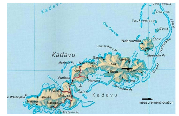
    [19] The Editors of Encyclopædia Britannica. Kadavu Island. Available from: https://www.britannica.com/place/Kadavu-Island.
    [20] Kadavu Map. Available from: http://nztourmaps.com/fiji_map_kadavu.htm.
    [21] Aukitino T, Khan M, Ahmed MR (2017) Wind energy resource assessment for Kiribati with a comparison of different methods of determining Weibull parameters. Energy Convers Manage 151: 641-660. doi: 10.1016/j.enconman.2017.09.027
    [22] Zhang MH (2015) Wind Resource Assesement and Micrositting : Science and Engineering. Singapore: John Wiley & Sons Singapore Pte. Ltd.
    [23] Fırtın E, Güler Ö, Akdağ SA (2011) Investigation of wind shear coefficients and their effect on electrical energy generation. Appl Energy 88: 4097-4105. doi: 10.1016/j.apenergy.2011.05.025
    [24] Gualtieri G, Secci S (2011) Wind shear coefficients, roughness length and energy yield over coastal locations in Southern Italy. Renewable Energy 36: 1081-1094. doi: 10.1016/j.renene.2010.09.001
    [25] Rehman S, Al-Abbadi NM (2008) Wind shear coefficient, turbulence intensity and wind power potential assessment for Dhulom, Saudi Arabia. Renewable Energy 33: 2653-2660. doi: 10.1016/j.renene.2008.02.012
    [26] Singh K, Bule L, Khan M, et al. (2019) Wind energy resource assessment for Vanuatu with accurate estimation of Weibull parameters. Energy Explor Exploit 37: 1804-1832. doi: 10.1177/0144598719866897
    [27] Justus CG, Hargraves WR, Mikhail A, et al. (1978) Methods for estimating wind speed distributions. J Appl Meteorolgy 17: 350-353. doi: 10.1175/1520-0450(1978)017<0350:MFEWSF>2.0.CO;2
    [28] Chaurasiya PK, Ahmed S, Warudkar V (2017) Study of different parameters estimation methods of Weibull distribution to determine wind power density using ground based Doppler SODAR instrument. Alexandria Eng J 55: 2299-2311.
    [29] Chaurasiya PK, Ahmed S, Warudkar V (2018) Comparative analysis of Weibull parameters for wind data measured from met-mast and remote sensing techniques. Renewable Energy 115: 1153-1165. doi: 10.1016/j.renene.2017.08.014
    [30] Rocha PAC, de Sousa RC, de Andrade CF, et al. (2012) Comparison of seven numerical methods for determining Weibull parameters for wind energy generation in the northeast region of Brazil. Appl Energy 89: 395-400. doi: 10.1016/j.apenergy.2011.08.003
    [31] Lysen E (1982) Introduction to wind energy: basic and advanced Introduction to wind energy with emphasis on water pumping windmills. Amersfoort: Consultancy services wind energy developing countries (CWD).
    [32] Ahmad S, Hussin W, Bawadi M, et al. (2003) Analysis of wind speed variations and estimation of Weibull parameters for wind power generation in Malaysia. 2nd Dubrovnik Conference on Sustainable Development of Energy, Water and Environment Systems, Dubrovnik, Croatia, 15-20 June, 61.
    [33] Katinas V, Marciukaitis M, Gecevicius G, et al. (2017) Statistical analysis of wind characteristics based on Weibull methods for estimation of power generation in Lithuania. Renewable Energy 113: 190-201. doi: 10.1016/j.renene.2017.05.071
    [34] Usta I, Arik I, Yenilmez I, et al. (2018) A new estimation approach based on moments for estimating Weibull parameters in wind power applications. Energy Convers Manage 164: 570-578. doi: 10.1016/j.enconman.2018.03.033
    [35] Arslan T, Bulut YM, Yavuz AA (2014) Comparative study of numerical methods for determining Weibull parameters for wind energy potential. Renewable Sustainable Energy Rev 40: 820-825. doi: 10.1016/j.rser.2014.08.009
    [36] Szafron C (2011) Wind energy conversion systems grid connection. Master's Thesis, Wroclaw University of Technology.
  • This article has been cited by:

    1. Ombeni John Mdee, Performance evaluation of Weibull analytical methods using several empirical methods for predicting wind speed distribution, 2020, 1556-7036, 1, 10.1080/15567036.2020.1832161
    2. Varadharajan Sankaralingam Sriraja Balaguru, Nesamony Jothi Swaroopan, Kannadasan Raju, Mohammed H. Alsharif, Mun-Kyeom Kim, Techno-Economic Investigation of Wind Energy Potential in Selected Sites with Uncertainty Factors, 2021, 13, 2071-1050, 2182, 10.3390/su13042182
    3. Ombeni JOHN, Evaluation of Rainfall Extreme Characteristics in Dodoma Urban, A Central Part of Tanzania, 2022, 9, 2148-9173, 166, 10.30897/ijegeo.1000458
    4. Krishneel A. Singh, M. G. M. Khan, Mohammed Rafiuddin Ahmed, Wind Energy Resource Assessment for Cook Islands With Accurate Estimation of Weibull Parameters Using Frequentist and Bayesian Methods, 2022, 10, 2169-3536, 25935, 10.1109/ACCESS.2022.3156933
    5. Mohammad Golam Mostafa Khan, Mohammed Rafiuddin Ahmed, Bayesian method for estimating Weibull parameters for wind resource assessment in a tropical region: a comparison between two-parameter and three-parameter Weibull distributions, 2023, 8, 2366-7451, 1277, 10.5194/wes-8-1277-2023
    6. Jean-Michel Soumien Kouadio, Franck Didier Néné, Moussa Grafouté, Alexandre N'guessan, Siaman Paule Carine Yeboua, N'goran Yao, Harnessing the wind energy potential in Yamoussoukro, the Economic Capital of Côte d'Ivoire, 2024, 10, 24058440, e30170, 10.1016/j.heliyon.2024.e30170
    7. Saiyad S. Kutty, M.G.M. Khan, M. Rafiuddin Ahmed, Analysis of wind characteristics and wind energy resource assessment for Tonga using eleven methods of estimating Weibull parameters, 2024, 10, 24058440, e30047, 10.1016/j.heliyon.2024.e30047
    8. Isaac D. Guedes Fialho, Eduardo San-Martin, Akihito Boa-Esperança, Feliciano José Ricardo Cangue, Vencislau Quissanga, Impact of guide vanes on the performance of Savonius wind turbines, 2025, 22, 1983-0882, e18014, 10.54033/cadpedv22n9-119
  • Reader Comments
  • © 2019 the Author(s), licensee AIMS Press. This is an open access article distributed under the terms of the Creative Commons Attribution License (http://creativecommons.org/licenses/by/4.0)
通讯作者: 陈斌, bchen63@163.com
  • 1. 

    沈阳化工大学材料科学与工程学院 沈阳 110142

  1. 本站搜索
  2. 百度学术搜索
  3. 万方数据库搜索
  4. CNKI搜索

Metrics

Article views(5624) PDF downloads(703) Cited by(8)

Figures and Tables

Figures(19)  /  Tables(8)

/

DownLoad:  Full-Size Img  PowerPoint
Return
Return

Catalog