This study detailed the course design principles and implementation of project-based learning (PBL) in a technology-themed graduate-level online course. Students were trained to develop knowledge and skills in instructional leadership, such as the capability to design, deliver, and evaluate educational technology professional development programs. Pre- and post- survey data were collected to examine any change in students' knowledge and skills in instructional leadership by completing this course (N = 18). Quantitative findings revealed positive learning outcomes, and there was statistical significance regarding student improvement in knowledge and skills of instructional leadership, rendering the PBL approach viable.
Citation: Min Lun Wu, Lan Li, Yuchun Zhou. Enhancing technology leaders' instructional leadership through a project-based learning online course[J]. STEM Education, 2023, 3(2): 89-102. doi: 10.3934/steme.2023007
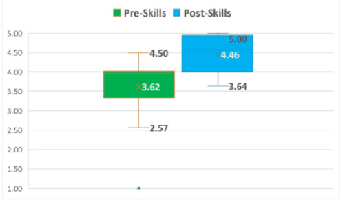
This study detailed the course design principles and implementation of project-based learning (PBL) in a technology-themed graduate-level online course. Students were trained to develop knowledge and skills in instructional leadership, such as the capability to design, deliver, and evaluate educational technology professional development programs. Pre- and post- survey data were collected to examine any change in students' knowledge and skills in instructional leadership by completing this course (N = 18). Quantitative findings revealed positive learning outcomes, and there was statistical significance regarding student improvement in knowledge and skills of instructional leadership, rendering the PBL approach viable.

| [1] |
Aas, M. and Paulsen, J.M., National strategy for supporting school principal's instructional leadership: A Scandinavian approach. Journal of Educational Administration, 2019, 57(5): 540‒553. https://doi.org/10.1108/JEA-09-2018-0168 doi: 10.1108/JEA-09-2018-0168

|
| [2] | Albritton, S. and Stacks, J., Implementing a Project-Based Learning Model in a Pre-Service Leadership Program. International Journal of Educational Leadership Preparation, 2016, 11(1): n1. |
| [3] |
Berkovich, I. and Hassan, T., Principals' digital instructional leadership during the pandemic: Impact on teachers' intrinsic motivation and students' learning. Educational Management Administration & Leadership, 2022, 17411432221113411. https://doi.org/10.1177/17411432221113411 doi: 10.1177/17411432221113411
|
| [4] |
Claassen, K., Dos Anjos, D.R., Kettschau, J. and Broding, H.C., How to evaluate digital leadership: a cross-sectional study. Journal of Occupational Medicine and Toxicology, 2021, 16(1): 1‒8. https://doi.org/10.1186/s12995-021-00335-x doi: 10.1186/s12995-020-00290-z
|
| [5] |
Dani, D.E., Wu, M.L., Hartman, S.L., Kessler, G., Grey, T.M.G., Liu, C., et al., Leveraging Partnerships to Support Community-Based Learning in a College of Education. Handbook of Research on Adult Learning in Higher Education, 2020, 58‒89. https://doi.org/10.4018/978-1-7998-1306-4.ch003 doi: 10.4018/978-1-7998-1306-4.ch003
|
| [6] | Edwards, B. and Hinueber, J., Why teachers make good learning leaders. The Learning Professional, 2015, 36(5): 26. |
| [7] | Elmore, R., Building a New Structure for School Leadership. Albert Shanker Institute. 2000. |
| [8] |
Helle, L., Tynjala, P. and Olkinurora, E., Project-based learning in post-secondary education: Theory, practice and rubber sling shots. Higher Education, 2006, 51: 287‒314. https://doi.org/10.1007/s10734-004-6386-5 doi: 10.1007/s10734-004-6386-5
|
| [9] | Jaipal-Jamani, K., Figg, C., Collier, D., Gallagher, T., Winters, K.L. and Ciampa, K., Developing TPACK of university faculty through technology leadership roles. Italian Journal of Educational Technology, 2018, 26(1): 39‒55. |
| [10] |
King, B. and Smith, C., Using project-based learning to develop teachers for leadership. The Clearing House: A Journal of Educational Strategies, Issues and Ideas, 2020, 93(3): 158‒164. https://doi.org/10.1080/00098655.2020.1735289 doi: 10.1080/00098655.2020.1735289
|
| [11] |
Lambrecht, J., Lenkeit, J., Hartmann, A., Ehlert, A., Knigge, M. and Spörer, N., The effect of school leadership on implementing inclusive education: How transformational and instructional leadership practices affect individualized education planning. International Journal of Inclusive Education, 2022, 26(9): 943‒957. https://doi.org/10.1080/13603116.2020.1752825 doi: 10.1080/13603116.2020.1752825
|
| [12] | Larmer, J., Mergendoller, J. and Boss, S., Setting the standard for project-based learning: A proven approach to rigorous classroom instruction. Alexandria, VA: Association for Supervision and Curriculum Development. 2015. |
| [13] |
Raman, A. and Thannimalai, R., Importance of technology leadership for technology integration: Gender and professional development perspective. SAGE Open, 2019, 9(4): 2158244019893707. https://doi.org/10.1177/2158244019893707 doi: 10.1177/2158244019893707
|
| [14] | Shadish, W.R., Cook, T.D. and Campbell, D.T., Experimental and quasi-experimental designs for generalized causal inference. Houghton, Mifflin and Company. 2002. |
| [15] |
Shaked, H., Perceptions of Israeli school principals regarding the knowledge needed for instructional leadership. Educational Management Administration & Leadership, 2023, 51(3): 655‒672. https://doi.org/10.1177/17411432211006092 doi: 10.1177/17411432211006092
|
| [16] |
Suyudi, M., Rahmatullah, A.S., Rachmawati, Y. and Hariyati, N., The Effect of Instructional Leadership and Creative Teaching on Student Actualization: Student Satisfaction as a Mediator Variable. International Journal of Instruction, 2022, 15(1): 113‒134. https://doi.org/10.29333/iji.2022.1517a doi: 10.29333/iji.2022.1517a
|
| [17] | Ylimaki, R.M., The New Instructional Leadership. Routledge. New York, NY. 2014. https://doi.org/10.4324/9780203112885 |

Figures(2) / Tables(3)
Min Lun Wu, Lan Li, Yuchun Zhou. Enhancing technology leaders' instructional leadership through a project-based learning online course[J]. STEM Education, 2023, 3(2): 89-102. doi: 10.3934/steme.2023007


 DownLoad: