Loading [MathJax]/jax/output/SVG/jax.js

An explicit finite volume algorithm for vanishing viscosity solutions on a network

  • In [Andreianov, Coclite, Donadello, Discrete Contin. Dyn. Syst. A, 2017], a finite volume scheme was introduced for computing vanishing viscosity solutions on a single-junction network, and convergence to the vanishing viscosity solution was proven. This problem models m incoming and n outgoing roads that meet at a single junction. On each road the vehicle density evolves according to a scalar conservation law, and the requirements for joining the solutions at the junction are defined via the so-called vanishing viscosity germ. The algorithm mentioned above processes the junction in an implicit manner. We propose an explicit version of the algorithm. It differs only in the way that the junction is processed. We prove that the approximations converge to the unique entropy solution of the associated Cauchy problem.

    Citation: John D. Towers. An explicit finite volume algorithm for vanishing viscosity solutions on a network[J]. Networks and Heterogeneous Media, 2022, 17(1): 1-13. doi: 10.3934/nhm.2021021

    Related Papers:

    [1] John D. Towers . An explicit finite volume algorithm for vanishing viscosity solutions on a network. Networks and Heterogeneous Media, 2022, 17(1): 1-13. doi: 10.3934/nhm.2021021
    [2] Boris Andreianov, Kenneth H. Karlsen, Nils H. Risebro . On vanishing viscosity approximation of conservation laws with discontinuous flux. Networks and Heterogeneous Media, 2010, 5(3): 617-633. doi: 10.3934/nhm.2010.5.617
    [3] Giuseppe Maria Coclite, Carlotta Donadello . Vanishing viscosity on a star-shaped graph under general transmission conditions at the node. Networks and Heterogeneous Media, 2020, 15(2): 197-213. doi: 10.3934/nhm.2020009
    [4] Markus Musch, Ulrik Skre Fjordholm, Nils Henrik Risebro . Well-posedness theory for nonlinear scalar conservation laws on networks. Networks and Heterogeneous Media, 2022, 17(1): 101-128. doi: 10.3934/nhm.2021025
    [5] Giuseppe Maria Coclite, Nicola De Nitti, Mauro Garavello, Francesca Marcellini . Vanishing viscosity for a $ 2\times 2 $ system modeling congested vehicular traffic. Networks and Heterogeneous Media, 2021, 16(3): 413-426. doi: 10.3934/nhm.2021011
    [6] Karoline Disser, Matthias Liero . On gradient structures for Markov chains and the passage to Wasserstein gradient flows. Networks and Heterogeneous Media, 2015, 10(2): 233-253. doi: 10.3934/nhm.2015.10.233
    [7] Wen Shen . Traveling wave profiles for a Follow-the-Leader model for traffic flow with rough road condition. Networks and Heterogeneous Media, 2018, 13(3): 449-478. doi: 10.3934/nhm.2018020
    [8] Giuseppe Maria Coclite, Lorenzo di Ruvo, Jan Ernest, Siddhartha Mishra . Convergence of vanishing capillarity approximations for scalar conservation laws with discontinuous fluxes. Networks and Heterogeneous Media, 2013, 8(4): 969-984. doi: 10.3934/nhm.2013.8.969
    [9] Abraham Sylla . Influence of a slow moving vehicle on traffic: Well-posedness and approximation for a mildly nonlocal model. Networks and Heterogeneous Media, 2021, 16(2): 221-256. doi: 10.3934/nhm.2021005
    [10] Christophe Chalons, Paola Goatin, Nicolas Seguin . General constrained conservation laws. Application to pedestrian flow modeling. Networks and Heterogeneous Media, 2013, 8(2): 433-463. doi: 10.3934/nhm.2013.8.433
  • In [Andreianov, Coclite, Donadello, Discrete Contin. Dyn. Syst. A, 2017], a finite volume scheme was introduced for computing vanishing viscosity solutions on a single-junction network, and convergence to the vanishing viscosity solution was proven. This problem models m incoming and n outgoing roads that meet at a single junction. On each road the vehicle density evolves according to a scalar conservation law, and the requirements for joining the solutions at the junction are defined via the so-called vanishing viscosity germ. The algorithm mentioned above processes the junction in an implicit manner. We propose an explicit version of the algorithm. It differs only in the way that the junction is processed. We prove that the approximations converge to the unique entropy solution of the associated Cauchy problem.


    This paper proposes an explicit finite volume scheme for first-order scalar conservation laws on a network having a single junction. The algorithm and analysis extend readily to networks with multiple junctions, due to the finite speed of propagation of the solutions of conservation laws. For the sake of concreteness, we view the setup as a model of traffic flow, with the vector of unknowns representing the vehicle density on each road. A number of such scalar models have been proposed, mostly differing in how the junction is modeled. An incomplete list of such models can be found in [4,5,6,7,8,11,12,13,14,15,16,18,19]. In this paper we focus on the so-called vanishing viscosity solution proposed and analyzed in [7] and [2]. The junction has m incoming and n outgoing roads. With uh denoting the density of vehicles on road h, and fh() denoting the flux on road h, on each road traffic evolves according to the Lighthill-Witham-Richards model

    tuh+xfh(uh)=0,h=1,,m+n. (1.1)

    Incoming roads are indexed by i{1,,m}, and outgoing roads by j{m+1,m+n}. Each road has a spatial domain denoted by Ωh, where Ωi=(,0) for i{1,,m} and Ωj=(0,) for j{m+1,m+n}. The symbol Γ is used to denote the spatial domain defined by the network of roads, and L(Γ×R+;[0,R]m+n) denotes the set of vectors u=(u1,,um+n) of functions satisfying

    uiL(R×R+;[0,R]),i{1,,m},ujL(R+×R+;[0,R]),j{m+1,,m+n}. (1.2)

    Following [2] we make the following assumptions concerning the fluxes fh.

    (A.1) For each h{1,,m+n}, fhLip([0,R];R+), and fhLh. Each fh satisfies fh(0)=fh(R)=0 and is unimodal (bell-shaped), meaning that for some ˉuh(0,R) fh(u)(ˉuhu)>0 for a.e. u[0,R].

    (A.2) For each h{1,,m+n}, fh is not linearly degenerate, meaning that fh is not constant on any nontrivial subinterval of [0,R].

    The study of vanishing viscosity solutions on a network was initiated by Coclite and Garavello [7], who proved that vanishing viscosity solutions converge to weak solutions if n=m and all of the fluxes fh are the same. Andreianov, Coclite and Donadello [2] proved well-posedness of the more general problem discussed in this paper, relying upon a generalization of recent results concerning conservation laws with discontinuous flux [1,3].

    For the convenience of the reader, and to establish notation, we review some relevant portions of the theory of network vanishing viscosity solutions, as described in [2], where we refer the reader for a more complete development. Let Gh(,) denote the Godunov flux associated with fh():

    Gh(β,α)={minz[α,β]fh(z),αβ,maxz[β,α]fh(z),βα. (1.3)

    (Compared to [2], we list the arguments α, β of Gh in reversed order.) Note that Gh is consistent, i.e., Gh(α,α)=fh(α). Also, Gh(,) is a nonincreasing (nondecreasing) function of its first (second) argument, is Lipschitz continuous with respect to each argument, i.e., for α,β[0,R] there exists Lh>0 such that

    LhGh(β,α)/β0,0Gh(β,α)/αLh,h{1,,m+n}. (1.4)

    Definition 1.1 (Vanishing viscosity germ [2]). The vanishing viscosity germ GVV is the subset of [0,R]m+n consisting of vectors u=(u1,,um+n) such that for some pu[0,R] there holds

    mi=1Gi(pu,ui)=m+nj=m+1Gj(uj,pu),Gi(pu,ui)=fi(ui),i=1,,m,Gj(uj,pu)=fj(uj),j=m+1,,m+n. (1.5)

    The definition of entropy solution requires one-sided traces along the half-line x=0 in R×R+. Thanks to Assumption A.2, the existence of strong traces at x=0 in the L1loc sense is guaranteed [20]. The traces are denoted

    γiui()=ui(,0),i{1,,m},γjuj()=uj(,0+),j{m+1,,m+n}. (1.6)

    Definition 1.2 (GVV-entropy solution [2]). Define qh:[0,R]2R:

    qh(v,w)=sign(vw)(fh(v)fh(w)),h=1,,m+n. (1.7)

    Given an initial condition u0L(Γ;[0,R]m+n), a vector u=(u1,,um+n) in L(Γ×R+;[0,R]m+n) is a GVV entropy solution associated with u0 if it satisfies the following conditions:

    ● For each h{1,,m+n}, each c[0,R], and any test function ξD(Ωh×R;R+),

    R+Ωh(|uhc|tξ+qh(uh,c)xξ)dxdt+Ωh|uh,0c|ξ(x,0)dx0. (1.8)

    ● For a.e. tR+, the vector of traces at the junction

    γu(t):=(γ1u1(t),,γm+num+n(t)) belongs to GVV.

    Associated with each kGVV, and allowing for a slight abuse of notation, one defines a road-wise constant stationary solution k(x) via

    kh(x)=kh,xΩh,h{1,,m+n}. (1.9)

    It is readily verified that viewed in this way, kh is a GVV-entropy solution. In fact all road-wise constant stationary solutions that are GVV-entropy solutions are associated with a kGVV in this manner.

    Definition 1.2 reveals the relationship between the set GVV and GVV-entropy solutions, and is well-suited to proving uniqueness of solutions. On the other hand, Definition 1.3 below is equivalent (Theorem 2.11 of [2]), and is better suited to proving that the limit of finite volume approximations is a GVV-entropy solution.

    Definition 1.3 (GVV-entropy solution [2]). Given an initial condition u0L(Γ;[0,R]m+n), a vector u=(u1,,um+n) in L(Γ×R+;[0,R]m+n) is a GVV entropy solution associated with u0 if it satisfies the following conditions:

    ● The first item of Definition 1.2 holds.

    ● For any kGVV, u satisfies the following Kružkov-type entropy inequality:

    m+nh=1(R+Ωh{|uhkh|ξt+qh(uh,kh)ξx}dxdt)0 (1.10)

    for any nonnegative test function ξD(R×(0,)).

    Theorem 1.4 (Well posedness [2]). Given any initial datum

    u0=(u1,0,,um+n,0)L(Γ;[0,R]m+n), (1.11)

    there exists one and only one GVV-entropy solution uL(Γ×R+;[0,R]m+n) in the sense of Definition 1.2.

    In addition to the results above, reference [2] also includes a proof of existence of the associated Riemann problem. Based on the resulting Riemann solver, a Godunov finite volume algorithm is constructed in [2], which handles the interface in an implicit manner. This requires the solution of a single nonlinear equation at each time step. The resulting finite volume scheme generates approximations that are shown to converge to the unique GVV-entropy solution. Reference [21] validates the algorithm by comparing finite volume approximations with exact solutions of a collection of Riemann problems.

    The main contribution of the present paper is an explicit version of the finite volume scheme of [2]. It differs only in the processing of the junction. We place an artificial grid point at the junction, which is assigned an artificial density. The artificial density is evolved from one time level to the next in an explicit manner. Thus a nonlinear equation solver is not required. (However, we found that in certain cases accuracy can be improved by processing the junction implicitly on the first time step.) Like the finite volume scheme of [2], the new algorithm has the order preservation property and is well-balanced. This makes it possible to employ the analytical framework of [2], resulting in a proof that the approximations converge to the unique entropy solution of the associated Cauchy problem.

    In Section 2 we present our explicit finite volume scheme and prove convergence to a GVV-entropy solution. In Section 3 we discuss numerical experience with the new scheme, including one example. Appendix A contains a proof that a fixed point algorithm introduced in Section 2 converges.

    For a fixed spatial mesh size Δx, define the grid points x0=0 and

    x=(+1/2)Δx,{,2,1},x=(1/2)Δx,{1,2,}. (2.1)

    Each road Ωh is discretized according to

    Ωi=1I,I:=(xΔx/2,x+Δx/2]  for 1,Ωj=1I,I:=[xΔx/2,x+Δx/2) for  1. (2.2)

    Our discretization of the spatial domain Γ is identical to that of [2], but differs slightly in appearance since we prefer to use whole number indices for cell centers and fractional indices for cell boundaries. We use the following notation for the finite volume approximations:

    Uh,suh(x,ts),Z{0},Pspγu(ts). (2.3)

    We are somewhat artificially assigning a density, namely Ps, to the single grid point x0=0 where the junction is located. We view the junction as a grid cell with width zero. We advance Ps from one time level to the next in an explicit manner, without requiring a nonlinear equation solver. This is the novel aspect of our finite volume scheme.

    Remark 1. We make the association Pspγu(ts) because it is conceptually helpful. In fact, it is justified in the special case of a stationary solution of the scheme associated with kGVV; see the proof of Lemma 2.3. However, we do not attempt to prove that Pspγu(ts) when Δ0. Fortunately, the convergence proof does not rely on pointwise convergence of Ps as Δ0.

    The initial data are initialized via

    Uh,0=1ΔxIuh,0(x)dx,h{1,,m+n},P0[0,R]. (2.4)

    Note that P0 can be any conveniently chosen value lying in [0,R] (but see Remark 3 and Section 3). Recall that (2.3) introduced Uh,s only for Z{0}. We can simplify some of the formulas that follow by defining Uh,s0=Ps for each h{1,,m+n}. The finite volume scheme then advances the approximations from time level s to time level s+1 according to

    {Ps+1=Psλ(m+nj=m+1Gj(Uj,s1,Ps)mi=1Gi(Ps,Ui,s1)),Ui,s+1=Ui,sλ(Gi(Ui,s+1,Ui,s)Gi(Ui,s,Ui,s1)),i{1,,m},1,Uj,s+1=Uj,sλ(Gj(Uj,s+1,Uj,s)Gj(Uj,s,Uj,s1)),j{m+1,,m+n},1. (2.5)

    Define λ=Δt/Δx. When taking the limit Δ:=(Δx,Δt)0, we assume that λ is fixed. Let L=max{Lh|h{1,,m+n}}. In what follows we assume that the following CFL condition is satisfied:

    λ(m+n)L1. (2.6)

    If all of the fh are the same, i.e., fh()=f() for all h{1,,m+n}, then (2.6) can be replaced by the following less restrictive condition (see Remark 6):

    λmax(m,n)L1. (2.7)

    Remark 2. The algorithm (2.5) is an explicit version of the scheme of [2]. To recover the scheme of [2] from (2.5), one proceeds as follows:

    ● first substitute Ps for Ps+1 in the first equation of (2.5), and solve the resulting equation for Ps (the implicit part of the algorithm of [2]),

    ● then advance each Uh,s to the next time level using the second and third equations of (2.5) (recalling the notational convention Uh,s0=Ps).

    The equation mentioned above (after substituting Ps for Ps+1) is clearly equivalent to

    m+nj=m+1Gj(Uj,s1,Ps)=mi=1Gi(Ps,Ui,s1). (2.8)

    The implicit portion of the scheme of [2] consists of solving (2.8) for the unknown Ps. Lemma 2.3 of [2] guarantees that this equation has a solution, which can be found using, e.g., regula falsi.

    Remark 3. The convergence of the scheme (2.5) is unaffected by the choice of P0, as long as it lies in [0,R]. However the choice of P0 does affect accuracy, see Section 3. We found that accurate results are obtained when P0 is a solution to the s=0 version of (2.8). We also found this solution can be conveniently approximated by iterating the first equation of (2.5), i.e.,

    P0ν+1=P0νλ(m+nj=m+1Gj(Uj,01,P0ν)mi=1Gi(P0ν,Ui,01)). (2.9)

    Moreover, we found that this same fixed point iteration approach is a convenient way to solve (2.8) when implementing the implicit scheme of [2]. From this point of view the algorithm of this paper and the algorithm of [2] only differ in whether the first equation of (2.5) is iterated once, or iterated to (approximate) convergence. See Appendix A for a proof that the iterative scheme (2.9) converges to a solution of (2.8).

    Remark 4. The CFL condition associated with the finite volume scheme of [2] is

    λL1/2. (2.10)

    As soon as there are more than a few roads impinging on the junction, our CFL condition (2.6) imposes a more severe restriction on the allowable time step, which becomes increasingly restrictive as more roads are included. One could view this as the price to be paid for the simplified processing of the junction. On the other hand, most of the specific examples discussed in the literature are limited to max(m,n)=2. In that case, if also all of the fh are the same, then (2.7) and (2.10) are equivalent. Finally, at the cost of some additional complexity, one could use a larger spatial mesh adjacent to the junction, which would allow for larger time steps. We do not pursue that here.

    Let χ(x) denote the characteristic function of the spatial interval I, and let χs(t) denote the characteristic function of the temporal interval [sΔt,(s+1)Δt). We extend the grid functions to functions defined on Ω×R+ via

    ui,Δ=s01χ(x)χs(t)Ui,s,i{1,,m},uj,Δ=s01χ(x)χs(t)Uj,s,j{m+1,,m+n}. (2.11)

    The discrete solution operator is denoted by SΔ, which operates according to

    SΔu0=(ui,Δ,,um,Δ,um+1,Δ,um+n,Δ). (2.12)

    The symbol Γdiscr is used to denote the spatial grid (excluding the artificial grid point associated with =0):

    Γdiscr=({1,,m}×{Z,1})({m+1,,m+n}×{Z,1}), (2.13)

    and with the notation

    Us=(Uh,s)(h,l)Γdiscr, (2.14)

    (Us,Ps) denotes the grid function generated by the scheme at time step s.

    Remark 5. In the case where m=n=1, i.e., a one-to-one junction, and f1f2, we have the special case of a conservation law with a spatially discontinuous flux at x=0. If we redefine the grid so that xj=jΔx, and set Us0=Ps, the explicit finite volume scheme proposed here reduces to the Godunov scheme first proposed in [10]. In reference [17] it was proven that (for m=n=1) the scheme converges to the vanishing viscosity solution under more general assumptions about the flux than the unimodality condition imposed here.

    Lemma 2.1. Fix a time level s. Assume that Ps[0,R] and Uh,s[0,R] for each h{1,m+n}. Then each Uh,s+1 is a nondecreasing function of each of its three arguments. Likewise, Ps+1 is a nondecreasing function of each of its m+n+1 arguments.

    Proof. For h{1,,m} and <1, or h{m+1,,m+n} and >1, the assertion about Uh,s+1 is a standard fact about three-point monotone schemes for scalar conservation laws [9]. For the remaining cases, we show that the relevant partial derivatives are nonnegative.

    Fix i{1,,m}, let =1. The partial derivatives of Ui,s+11 are

    Ui,s+11/Ui,s2=λGi(Ui,s1,Ui,s2)/Ui,s2,Ui,s+11/Ui,s0=λGi(Ui,s0,Ui,s1)/Ui,s0,Ui,s+11/Ui,s1=1λGi(Ui,s0,Ui,s1)/Ui,s1+λGi(Ui,s1,Ui,s0)/Ui,s1. (2.15)

    That partial derivatives in the first two lines are nonnegative is a well-known property of the Godunov numerical flux. The partial derivative on the third line is nonnegative due to (1.4) and the CFL condition (2.6).

    A similar calculation shows that the partial derivatives of Uj,s+11 are nonnegative, for each j{m+1,,m+n}.

    It remains to show that the partial derivatives of Ps+1 are all nonnegative. Note that Ps+1 is a function of Ps, along with Ui,s1 for i{1,,m}, and Uj,s1 for j{m+1,,m+n}. The partial derivatives of Ps+1 are

    Ps+1/Ui,s1=λGi(Ps,Ui,s1)/Ui,s1,Ps+1/Uj,s1=λGj(Uj,s1,Ps)/Uj,s1,Ps+1/Ps=1λ(m+nj=m+1Gj(Uj,s1,Ps)/Psmi=1Gi(Ps,Ui,s1)/Ps)1λ(m+nj=m+1max(0,fj(Ps))mi=1min(0,fi(Ps))). (2.16)

    The first two partial derivatives are clearly nonnegative. For the third partial derivative we have used the following readily verified fact about the Godunov flux:

    min(0,fh(β))Ghβ(β,α)0Ghα(β,α)max(0,fh(α)), (2.17)

    and thus the third partial derivative is nonnegative due to (1.4) and the CFL condition (2.6).

    Remark 6. If all of the fluxes fh=f are the same, then the bound above for Ps+1/Ps simplifies to

    Ps+1/Ps1λ(nmax(0,f(Ps))mmin(0,f(Ps))), (2.18)

    from which it is clear that Ps+1/Ps0 under the less restrictive CFL condition (2.7).

    Lemma 2.2. Assuming that the initial data satisfies u0L(Γ;[0,R]m+n), the finite volume approximations satisfy Uh,s[0,R], Ps[0,R] for s0.

    Proof. The assertion is true for s=0, due to our method of discretizing the initial data. Define a pair of grid functions (˜U,˜P) and (ˆU,ˆP):

    ˜Uh=0,˜P=0,ˆUh=R,ˆP=R. (2.19)

    It is readily verified that (˜U,˜P) and (ˆU,ˆP) are stationary solutions of the finite volume scheme, and we have

    ˜UhU0,hˆUh,˜PP0ˆP. (2.20)

    After an application of a single step of the finite volume scheme, these ordering relationships are preserved, as a result of Lemma 2.1. Since (˜U,˜P) and (ˆU,ˆP) remain unchanged after applying the finite volume scheme, we have

    ˜UhU1,hˆUh,˜PP1ˆP. (2.21)

    This proves the assertion for s=1, and makes it clear that the proof can be completed by continuing this way by induction on s.

    Given kGVV, we define a discretized version (K,P) with K=(Kh)(h,l)Γdiscr where

    Kh={ki,<0  and h{1,,m},kj,>0  and  h{m+1,,m+n}. (2.22)

    and P=pk. Here pk denotes the value of p associated with k whose existence is stated in Definition 1.1.

    Lemma 2.3. The finite volume scheme of Section 2 is well-balanced in the sense that each (K,P) associated with kGVV as above is a stationary solution of the finite volume scheme.

    Proof. For each fixed h, and ||>1, the scheme reduces to the classical Godunov scheme without any involvement of the junction, and thus {Kh}||>1 is clearly unchanged by application of the scheme in this case.

    Fix i{1,,m}, and take =1. When the scheme is applied in order to advance Ki1=ki to the next time level, the result is

    kiλ(Gi(pk,ki)Gi(ki,ki))=kiλ(fi(ki)fi(ki))=ki. (2.23)

    Here we have used the definition of pk, along with the consistency of the Godunov flux, Gi(α,α)=fi(α). Similarly, when j{m+1,,m+n} is fixed, and the scheme is applied at =1, the result is kj. It remains to show that the scheme leaves P unchanged. The quantity P=pk is advanced to the next time level according to

    pkλ(nj=m+1Gj(kj,pk)mi=1Gi(pk,ki))=pk, (2.24)

    where we have applied the first equation of (1.5).

    With the notation ab=max(a,b) and ab=min(a,b), define

    Qh+1/2[Us,ˆUs]=Gh(Uh,s+1ˆUh,s+1,Uh,sˆUh,s)Gh(Uh,s+1ˆUh,s+1,Uh,sˆUh,s). (2.25)

    Lemma 2.4. Let 0ξD(R×(0,)), and define ξs=ξ(x,ts). Given any initial conditions u0,ˆu0L(Γ;[0,R]m+n), the associated finite volume approximations satisfy the following discrete Kato inequality:

    mi=1ΔxΔt+s=1<0|Ui,sˆUi,s|(ξsξs1)/Δt+mi=1ΔxΔt+s=00Qi1/2[Us,ˆUs](ξsξs1)/Δx+m+nj=m+1ΔxΔt+s=1>0|Ui,sˆUi,s|(ξsξs1)/Δt+m+nj=m+1ΔxΔt+s=00Qj+1/2[Us,ˆUs](ξs+1ξs)/Δx+ΔxΔt+s=1|PsˆPs|(ξs0ξs10)/Δt0. (2.26)

    Proof. From the monotonicity property (Lemma 2.1), a standard calculation [9] yields

    |Ui,s+1ˆUi,s+1||Ui,sˆUi,s|λ(Qi+1/2[Us,ˆUs]Qi1/2[Us,ˆUs]),1,i{1,,m},|Uj,s+1ˆUj,s+1||Uj,sˆUj,s|λ(Qj+1/2[Us,ˆUs]Qj1/2[Us,ˆUs]),1,j{m+1,,m+n},|Ps+1ˆPs+1||PsˆPs|λ(m+nj=m+1Qj1/2[Us,ˆUs]mi=1Qi1/2[Us,ˆUs]). (2.27)

    We first multiply each of the first and second set of inequalities indexed by Δxξs. Likewise, we multiply each of the last set of inequalities by Δxξs0. Next we sum the inequalities indexed by i over i{1,,m}, s0, 1, and then sum by parts in s and . Similarly, we sum the inequalities indexed by j over j{m+1,,m+n}, s0, 1, and then sum by parts in s and . For the last set of inequalities we sum over s0, and then sum by parts in s. When all of the sums are combined the result is (2.26).

    Lemma 2.5. Suppose that u is a subsequential limit of the finite volume approximations SΔu0 generated by the scheme of Section 2. Then u is a GVV entropy solution.

    Proof. The proof that the first condition of Definition 1.2 holds is a slight adaptation of a standard fact about monotone schemes for scalar conservation laws [9].

    The proof is completed by verifying the second condition of Definition 1.2. Let kGVV, with k also denoting (by a slight abuse of notation) the associated road-wise constant GVV solution. Following [2], we invoke Lemma 2.4, with ˆu=k, and rely on the fact that SΔk is a stationary solution of the finite volume scheme (Lemma 2.3). When Δ0 in the resulting version of (2.26), the result is the desired Kružkov-type entropy inequality (1.10). The crucial observation here is that the last sum on the left side of (2.26) vanishes in the limit.

    With Lemmas 2.1 through 2.5 in hand it is possible to repeat the proof of Theorem 3.3 of [2], which yields Theorem 2.6 below.

    Theorem 2.6. For a given initial datum u0L(Γ;[0,Rm+n]), the finite volume scheme of Section 2 converges to the unique GVV-entropy solution u, i.e., SΔu0u as Δ0.

    We found that if P0 is initialized carefully the approximations generated by the explicit scheme of Section 2 differ only slightly from those generated by the implicit scheme of [2]. This conclusion is based on testing on the Riemann problems of [21], among others. Thus we limit our discussion to the initialization of P0, including one numerical example that illustrates the difference between a bad choice for P0 and a good one.

    Initialization of P0. As mentioned previously, convergence is guaranteed as long as P0[0,R], but the choice of P0 can affect accuracy. A bad choice of P0 can result in spurious numerical artifacts, more specifically "bumps" that travel away from x=0. These bumps have been noticed before in the case of a one-to-one junction, see Example 2 of [17]. We have found two approaches that are effective in initializing P0:

    ● Initialize P0 by solving the nonlinear equation (2.8) (with s=0). In other words, the scheme is implicit on the first time step, and explicit on all subsequent time steps. No spurious artifacts were observed with this method of initialization. For our numerical tests, we solved (2.8) via the iteration (2.9) purely as a matter of convenience, but regula falsi, as suggested in [2], may be more efficient.

    ● Initialize P0 by choosing P0=Ui,01 for some i{1,,m} or P0=Uj,01 for some j{m+1,,m+n}. If a spurious bump is observed, try a different choice from the same finite set. Obviously, this is a trial and error method, and may require re-running a simulation. Based on a substantial amount of experience with one-to-one junctions (discontinuous flux problems), there seems to always be a choice for which no spurious bump appears. This approach also seems to work for more general junctions (up to and including two-by-two), but our experience here is more limited.

    Example 1. This example demonstrates the appearance of a spurious bump when P0 is initialized with a "bad" value. We emphasize that convergence is not affected, only accuracy. This is a Riemann problem featuring a two-to-one merge junction. The initial data is (u1,0,u2,0,u3,0)=(3/4,4/5,1/5). See Figure 1. We used (Δx,Δt)=(.005,.0025), λ=1/2, for 25 time steps. In the left panel, we used P0=1/5. In the right panel, we computed P0 by the fixed point iteration (2.9), stopping when the difference was |P0k+1P0k|<106. In the left panel, a spurious bump in the graph of u2 left is visible. This numerical artifact is not visible in the right panel.

    Figure 1. 

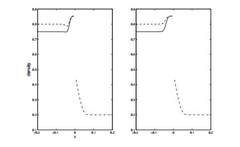
    Example 1. Left panel: P0=1/5. Right panel: P0 computed by the fixed point iteration (2.9), or by choosing P0=4/5. Solid line: u1, dashed line: u2, dot-dashed line: u3. In the left panel a spurious bump in u2 is visible, due to a bad choice of P0 (which does not affect convergence). In the right panel there is no spurious bump

    .

    One can also get rid of the spurious bump by choosing P0=4/5. With this choice we got results that are visually indistinguishable from those obtained when using (2.9) for P0.

    I thank two anonymous referees for their comments and suggestions.

    In this appendix we prove that the fixed point iterations (2.9) converge to a solution of the equation (2.8). Let p=Ps, and define the vector u=(u1,,um+n) by

    ui=Ui,s1fori=1,,m,uj=Uj,s1 for  j=m+1,,m+n. (A.1)

    Then (2.8) takes the form

    Φoutu(p)=Φinu(p), (A.2)

    where

    Φinu(p)=mi=1Gi(p,ui),Φoutu(p)=m+nj=m+1Gj(uj,p). (A.3)

    This notation agrees with that of [2], where it was shown that Φinu()Φoutu() changes from nonnegative to nonpositive over the interval [0,R], and thus the intermediate value theorem guarantees at least one solution of (A.2). Reference [2] suggested regula falsi as a method of locating such a solution. As an alternative we proposed the iterative method (2.9) because it clarifies the relationship between the finite volume algorithm of this paper and that of [2]. Moreover we found that our explicit finite volume scheme can be improved by using a hybrid method, where the implicit scheme of [2] is employed on the first time step and our explicit method is used on all later time steps. In that situation the iterative algorithm (2.9) was found to be a convenient way to implement the nonlinear equation solver that is required on the first time step.

    With the simplified notation introduced above, the iterative scheme (2.9) becomes

    pν+1=pνλ(Φoutu(pν)Φinu(pν)),p0[0,R]. (A.4)

    Proposition 1. The sequence {pν} produced by the iterative scheme (A.4) converges to a solution of (A.2).

    Proof. Note that pGi(p,ui) is nonincreasing on [0,R], pGj(uj,p) is nondecreasing on [0,R], and

    0Gi(0,ui),Gi(R,ui)=0,Gj(uj,0)=0,0Gj(uj,R). (A.5)

    Thus, pΦinu(p) is nonincreasing on [0,R], pΦoutu(p) is nondecreasing on [0,R], and

    0Φinu(0),Φinu(R)=0,Φoutu(0)=0,0Φoutu(R). (A.6)

    Define Ψu according to

    Ψu(p)=Φoutu(p)Φinu(p), (A.7)

    and observe that Ψu is Lipschitz continuous on [0,R] with Lipschitz constant bounded by (m+n)L. Also note that Ψu is nondecreasing on [0,R], and

    Ψu(0)0Ψu(R). (A.8)

    Define

    Π(p)=pλΨu(p). (A.9)

    Π is Lipschitz continuous and

    Π(p)=1λΨu(p)1λ(m+n)L. (A.10)

    Thanks to (A.10) and the CFL condition (2.6), it is clear that Π is nondecreasing on [0,R], and recalling (A.8) we have

    0Π(0)Π(p)Π(R)R for p[0,R]. (A.11)

    Thus Π maps [0,R] continuously into [0,R]. In terms of Π, the iterative scheme (A.4) is

    pν+1=Π(pν),p0[0,R]. (A.12)

    We can now prove convergence of the sequence {pν}. First take the case where pν0+1=pν0 for some ν0. Then pν=pν0 for νν0, so pνpν0. Also pν0+1=pν0 implies that Ψu(pν0)=0, and thus pν0 is a solution of (A.3).

    Now consider the case where pν+1pν for all ν0. Then

    pν+1pν=Π(pν)Π(pν1)=Π(pν)Π(pν1)pνpν1(pνpν1). (A.13)

    Since Π is nondecreasing and pνpν10, pν+1pν0, (A.13) implies that

    sign(pν+1pν)=sign(pνpν1)==sign(p1p0). (A.14)

    In other words, the sequence {pν} is monotonic. Since we also have {pν}[0,R], pν converges to some p[0,R], and it follows from continuity of Ψu that the limit p is a solution of (A.3).


    [1] On interface transmission conditions for conservation laws with discontinuous flux of general shape. J. Hyberbolic Differ. Equ. (2015) 12: 343-384.
    [2] Well-posedness for vanishing viscosity solutions of scalar conservation laws on a network. Discrete Contin. Dyn. Syst. - A (2017) 37: 5913-5942.
    [3] A theory of L1-dissipative solvers for scalar conservation laws with discontinuous flux. Arch. Ration. Mech. Anal. (2011) 201: 27-86.
    [4] Flows on networks: Recent results and perspectives. EMS Surv. Math. Sci. (2014) 1: 47-111.
    [5] Numerical approximations of a traffic flow model on networks. Netw. Heterog. Media (2006) 1: 57-84.
    [6] Vanishing viscosity on a star-shaped graph under general transmission conditions at the node. Netw. Heterog. Media (2020) 15: 197-213.
    [7] Vanishing viscosity for traffic flow on networks. SIAM J. Math. Anal. (2010) 42: 1761-1783.
    [8] Traffic flow on a road network. SIAM J. Math. Anal. (2005) 36: 1862-1886.
    [9] Monotone difference approximations for scalar conservation laws. Math. Comp. (1980) 34: 1-21.
    [10] On scalar conservation laws with point source and discontinuous flux function. SIAM J. Math. Anal. (1995) 26: 1425-1451.
    [11]

    U. S. Fjordholm, M. Musch and N. H. Risebro, Well-posedness theory for nonlinear scalar conservation laws on networks, preprint, https://arXiv.org/pdf/2102.06400.pdf.

    [12] Conservation laws on complex networks. Ann. Inst. H. Poincaré Anal. Non Linéare (2009) 26: 1925-1951.
    [13] Speed limit and ramp meter control for traffic flow networks. Eng. Optim. (2016) 48: 1121-1144.
    [14] Comparative study of macroscopic traffic flow models at road junctions. Netw. Heterog. Media (2020) 15: 216-279.
    [15] Phenomenological model for dynamic traffic flow in networks. Transp. Res. B (1995) 29: 407-431.
    [16] A mathematical model of traffic flow on a network of unidirectional roads. SIAM J. Math. Anal. (1995) 26: 999-1017.
    [17] Convergence of a Godunov scheme for for conservation laws with a discontinuous flux lacking the crossing condition. J. Hyperbolic Differ. Equ. (2017) 14: 671-701.
    [18]

    J. Lebacque, The Godunov scheme and what it means for first order traffic flow models, in Proceedings of the 13th International Symposium of Transportation and Traffic Theory (ed. J. Lesort), Elsevier, (1996), 647–677.

    [19] First order macroscopic traffic flow models for networks in the context of dynamic assignment. Transportation Planning and Applied Optimization (2004) 64: 119-140.
    [20] Existence of strong traces for quasi-solutions of multidimensional scalar conservation laws. J. Hyperbolic Differ. Equ. (2007) 4: 729-770.
    [21] On the implementation of a finite volumes scheme with monotone transmission conditions for scalar conservation laws on a star-shaped network. Appl. Numer. Math. (2020) 155: 181-191.
  • This article has been cited by:

    1. Nicola De Nitti, Enrique Zuazua, On the Controllability of Entropy Solutions of Scalar Conservation Laws at a Junction via Lyapunov Methods, 2023, 51, 2305-221X, 71, 10.1007/s10013-022-00598-9
    2. Michael Herty, Niklas Kolbe, Siegfried Müller, Central schemes for networked scalar conservation laws, 2022, 18, 1556-1801, 310, 10.3934/nhm.2023012
    3. Markus Musch, Ulrik Skre Fjordholm, Nils Henrik Risebro, Well-posedness theory for nonlinear scalar conservation laws on networks, 2022, 17, 1556-1801, 101, 10.3934/nhm.2021025
    4. Michael Herty, Niklas Kolbe, Siegfried Müller, A Central Scheme for Two Coupled Hyperbolic Systems, 2024, 6, 2096-6385, 2093, 10.1007/s42967-023-00306-5
    5. Dilip Sarkar, Shridhar Kumar, Pratibhamoy Das, Higinio Ramos, Higher-order convergence analysis for interior and boundary layers in a semi-linear reaction-diffusion system networked by a $ k $-star graph with non-smooth source terms, 2024, 19, 1556-1801, 1085, 10.3934/nhm.2024048
    6. Sabrina F. Pellegrino, A filtered Chebyshev spectral method for conservation laws on network, 2023, 151, 08981221, 418, 10.1016/j.camwa.2023.10.017
  • Reader Comments
  • © 2022 the Author(s), licensee AIMS Press. This is an open access article distributed under the terms of the Creative Commons Attribution License (http://creativecommons.org/licenses/by/4.0)
通讯作者: 陈斌, bchen63@163.com
  • 1. 

    沈阳化工大学材料科学与工程学院 沈阳 110142

  1. 本站搜索
  2. 百度学术搜索
  3. 万方数据库搜索
  4. CNKI搜索

Metrics

Article views(1890) PDF downloads(356) Cited by(6)

Figures and Tables

Figures(1)

Other Articles By Authors

/

DownLoad:  Full-Size Img  PowerPoint
Return
Return

Catalog