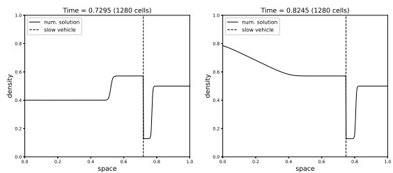
In this paper, we propose a macroscopic model that describes the influence of a slow moving large vehicle on road traffic. The model consists of a scalar conservation law with a nonlocal constraint on the flux. The constraint level depends on the trajectory of the slower vehicle which is given by an ODE depending on the downstream traffic density. After proving well-posedness, we first build a finite volume scheme and prove its convergence, and then investigate numerically this model by performing a series of tests. In particular, the link with the limit local problem of [M. L. Delle Monache and P. Goatin, J. Differ. Equ. 257 (2014), 4015–4029] is explored numerically.
Citation: Abraham Sylla. Influence of a slow moving vehicle on traffic: Well-posedness and approximation for a mildly nonlocal model[J]. Networks and Heterogeneous Media, 2021, 16(2): 221-256. doi: 10.3934/nhm.2021005
In this paper, we propose a macroscopic model that describes the influence of a slow moving large vehicle on road traffic. The model consists of a scalar conservation law with a nonlocal constraint on the flux. The constraint level depends on the trajectory of the slower vehicle which is given by an ODE depending on the downstream traffic density. After proving well-posedness, we first build a finite volume scheme and prove its convergence, and then investigate numerically this model by performing a series of tests. In particular, the link with the limit local problem of [M. L. Delle Monache and P. Goatin, J. Differ. Equ. 257 (2014), 4015–4029] is explored numerically.

| [1] |
Existence and nonexistence of TV bounds for scalar conservation laws with discontinuous flux. Comm. Pure Appl. Math (2011) 64: 84-115. 
|
| [2] |
Strong traces for averaged solutions of heterogeneous ultra-parabolic transport equations. J. Hyperbolic Differ. Equ. (2013) 10: 659-676.
|
| [3] |
Crowd dynamics and conservation laws with nonlocal constraints and capacity drop. Math. Models Methods in Appl. (2014) 24: 2685-2722.
|
| [4] |
Qualitative behaviour and numerical approximation of solutions to conservation laws with non-local point constraints on the flux and modeling of crowd dynamics at the bottlenecks. ESAIM: M2AN (2016) 50: 1269-1287.
|
| [5] |
Analysis and approximation of one-dimensional scalar conservation laws with general point constraints on the flux. J. Math. Pures et Appl. (2018) 116: 309-346.
|
| [6] |
Finite volume schemes for locally constrained conservation laws. Numer. Math. (2010) 115: 609-645.
|
| [7] |
A theory of $\text{L}^{1}$-dissipative solvers for scalar conservation laws with discontinuous flux. Arch. Ration. Mech. Anal. (2011) 201: 27-86.
|
| [8] |
Kružkov's estimates for scalar conservation laws revisited. Trans. Amer. Math. Soc. (1998) 350: 2847-2870.
|
| [9] | Two algorithms for a fully coupled and consistently macroscopic PDE-ODE system modeling a moving bottleneck on a road. Math. Eng. (2018) 1: 55-83. |
| [10] |
A family of numerical schemes for kinematic flows with discontinuous flux. J. Engrg. Math. (2008) 60: 387-425.
|
| [11] |
An Engquist-Osher-type scheme for conservation laws with discontinuous flux adapted to flux connections. SIAM J. Numer. Anal. (2009) 47: 1684-1712.
|
| [12] |
On the time continuity of entropy solutions. J. Evol. Equ. (2011) 11: 43-55.
|
| [13] |
Error estimate for Godunov approximation of locally constrained conservation laws. SIAM J. Numer. Anal. (2012) 50: 3036-3060.
|
| [14] |
A conservative scheme for non-classical solutions to a strongly coupled PDE-ODE problem. Interfaces Free Bound. (2017) 19: 553-570.
|
| [15] |
General constrained conservation laws. Application to pedestrian flow modeling. Networks Heterogen. Media (2013) 8: 433-463.
|
| [16] |
A non-local traffic flow model for 1-to-1 junctions. European Journal of Applied Mathematics (2020) 31: 1029-1049.
|
| [17] |
A well posed conservation law with a variable unilateral constraint. J. Differ. Equ. (2007) 234: 654-675.
|
| [18] |
Stability and total variation estimates on general scalar balance laws. Commun. Math. Sci. (2009) 7: 37-65.
|
| [19] |
Pedestrian flows and non-classical shocks. Math. Methods Appl. Sci. (2005) 28: 1553-1567.
|
| [20] |
Scalar conservation laws with moving constraints arising in traffic flow modeling: An existence result. J. Differ. Equ. (2014) 257: 4015-4029.
|
| [21] |
Stability estimates for scalar conservation laws with moving flux constraints. Networks Heterogen. Media (2017) 12: 245-258.
|
| [22] |
Uniform-in-time convergence result of numerical methods for non-linear parabolic equations. Numer. Math. (2016) 132: 721-766.
|
| [23] | R. Eymard, T. Gallouët and R. Herbin, Finite Volume Methods, North-Holland, Amsterdam, 2000. |
| [24] |
H. Helge and H. Risebro, Front Tracking for Hyperbolic Conservation Laws, Springer-Verlag, New York, 2002. doi: 10.1007/978-3-642-56139-9
|
| [25] | First order quasilinear equations with several independent variables. Mat. Sb. (N.S.) (1970) 81: 228-255. |
| [26] |
Moving bottlenecks in car traffic flow: A PDE-ODE coupled model. SIAM J. Math. Analysis (2011) 43: 50-67.
|
| [27] |
Well-Posedness for scalar conservation laws with moving flux constraints. SIAM J. Appl. Math. (2018) 79: 641-667.
|
| [28] | T. Liard and B. Piccoli, On entropic solutions to conservation laws coupled with moving bottlenecks, preprint, hal-02149946. |
| [29] |
Strong traces for conservation laws with general non-autonomous flux. SIAM J. Math. Analysis (2018) 50: 6049-6081.
|
| [30] |
On the strong pre-compactness property for entropy solutions of a degenerate elliptic equation with discontinuous flux. J. Differ. Equ. (2009) 247: 2821-2870.
|
| [31] |
Existence and strong pre-compactness properties for entropy solutions of a first-order quasilinear equation with discontinuous flux. Arch. Ration. Mech. Anal. (2010) 195: 643-673.
|
| [32] |
Convergence of the Godunov scheme for a scalar conservation law with time and space discontinuities. J. Hyperbolic Differ. Equ. (2018) 15: 175-190.
|
| [33] |
Convergence via OSLC of the Godunov scheme for a scalar conservation law with time and space flux discontinuities. Numer. Math. (2018) 139: 939-969.
|
Figures(5) / Tables(3)
Abraham Sylla. Influence of a slow moving vehicle on traffic: Well-posedness and approximation for a mildly nonlocal model[J]. Networks and Heterogeneous Media, 2021, 16(2): 221-256. doi: 10.3934/nhm.2021005


 DownLoad: