Comparative study of macroscopic traffic flow models at road junctions

Paola Goatin; Elena Rossi; Paola Goatin; Elena Rossi

doi:10.3934/nhm.2020012

Networks and Heterogeneous Media

2020, Volume 15, Issue 2: 261-279. doi: 10.3934/nhm.2020012

Previous Article Next Article

Comparative study of macroscopic traffic flow models at road junctions

Paola Goatin ^{1
,},
Elena Rossi ^{2
,
,}

1.
Inria Sophia Antipolis - Méditerranée, Université Côte d'Azur, Inria, CNRS, LJAD, 2004 route des Lucioles - BP 93, 06902 Sophia Antipolis Cedex, France
2.
Università degli Studi di Milano-Bicocca, Dipartimento di Matematica e Applicazioni, via R. Cozzi 55, 20126 Milano, Italy

Received: 01 February 2020 Published: 30 April 2020
Primary: 35L65, 90B20; Secondary: 82B21

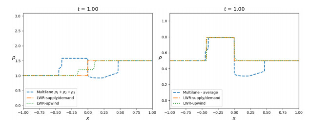
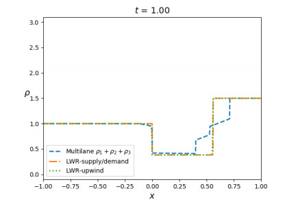
We qualitatively compare the solutions of a multilane model with those produced by the classical Lighthill-Whitham-Richards equation with suitable coupling conditions at simple road junctions. The numerical simulations are based on the Godunov and upwind schemes. Several tests illustrate the models' behaviour in different realistic situations.
- Macroscopic traffic flow models on networks,
- multilane models,
- multi-population models,
- finite volume schemes,
- hyperbolic systems of balance laws
Citation: Paola Goatin, Elena Rossi. Comparative study of macroscopic traffic flow models at road junctions[J]. Networks and Heterogeneous Media, 2020, 15(2): 261-279. doi: 10.3934/nhm.2020012

Related Papers:

Abstract

We qualitatively compare the solutions of a multilane model with those produced by the classical Lighthill-Whitham-Richards equation with suitable coupling conditions at simple road junctions. The numerical simulations are based on the Godunov and upwind schemes. Several tests illustrate the models' behaviour in different realistic situations.

References

[1]	Adimurthi and G. D. V. Gowda, Conservation law with discontinuous flux, J. Math. Kyoto Univ., 43 (2003), 27–70. doi: 10.1215/kjm/1250283740
[2]	Godunov-type methods for conservation laws with a flux function discontinuous in space. SIAM J. Numer. Anal. (2004) 42: 179-208.
[3]	Optimal entropy solutions for conservation laws with discontinuous flux-functions. J. Hyperbolic Differ. Equ. (2005) 2: 783-837.
[4]	Traffic flow on a road network. SIAM J. Math. Anal. (2005) 36: 1862-1886.
[5]	A destination-preserving model for simulating Wardrop equilibria in traffic flow on networks. Netw. Heterog. Media (2015) 10: 857-876.
[6]	On scalar conservation laws with point source and discontinuous flux function. SIAM J. Math. Anal. (1995) 26: 1425-1451.
[7]	Scalar conservation laws with discontinuous flux function. I. The viscous profile condition. Comm. Math. Phys. (1996) 176: 23-44.
[8]	A. Festa and P. Goatin, Modeling the impact of on-line navigation devices in traffic flows, 2019 IEEE 58th Conference on Decision and Control (CDC), Nice, France (2019), 323–328. doi: 10.1109/CDC40024.2019.9030208
[9]	M. Garavello, K. Han and B. Piccoli, Models for Vehicular Traffic on Networks, AIMS Series on Applied Mathematics, 9, American Institute of Mathematical Sciences (AIMS), Springfield, MO, 2016.
[10]	Source-destination flow on a road network. Commun. Math. Sci. (2005) 3: 261-283.
[11]	M. Garavello and B. Piccoli, Traffic Flow on Networks. Conservation Laws Models, AIMS Series on Applied Mathematics, 1, American Institute of Mathematical Sciences (AIMS), Springfield, MO, 2006.
[12]	Solution of the Cauchy problem for a conservation law with a discontinuous flux function. SIAM J. Math. Anal. (1992) 23: 635-648.
[13]	Speed limit and ramp meter control for traffic flow networks. Eng. Optim. (2016) 48: 1121-1144.
[14]	A multiLane macroscopic traffic flow model for simple networks. SIAM J. Appl. Math. (2019) 79: 1967-1989.
[15]	A mathematical model of traffic flow on a network of unidirectional roads. SIAM J. Math. Anal. (1995) 26: 999-1017.
[16]	H. Holden and N. H. Risebro, Front Tracking for Hyperbolic Conservation Laws, Applied Mathematical Sciences, 152, Springer, Heidelberg, 2015. doi: 10.1007/978-3-662-47507-2
[17]	Models for dense multilane vehicular traffic. SIAM J. Math. Anal. (2019) 51: 3694-3713.
[18]	K. H. Karlsen, N. H. Risebro and J. D. Towers, $L^1$stability for entropy solutions of nonlinear degenerate parabolic convection-diffusion equations with discontinuous coefficients, Skr. K. Nor. Vidensk. Selsk., (2003), 1–49.
[19]	On kinematic waves. II. A theory of traffic flow on long crowded roads. Proc. Roy. Soc. London. Ser. A. (1955) 229: 317-345.
[20]	Shock waves on the highway. Operations Res. (1956) 4: 42-51.
[21]	Discrete-time system optimal dynamic traffic assignment (SO-DTA) with partial control for physical queuing networks. Transportation Science (2018) 52: 982-1001.
[22]	A multilane junction model. TRANSPORTMETRICA (2012) 8: 243-260.
[23]	Convergence of a difference scheme for conservation laws with a discontinuous flux. SIAM J. Numer. Anal. (2000) 38: 681-698.

Reader Comments

Your name:*

Email:*
© 2020 the Author(s), licensee AIMS Press. This is an open access article distributed under the terms of the Creative Commons Attribution License (http://creativecommons.org/licenses/by/4.0)