Root colonization dynamics of alginate encapsulated rhizobacteria: implications for <i>Arabidopsis thaliana</i> root growth and durum wheat performance

Amel Balla; Allaoua Silini; Hafsa Cherif-Silini; Francesca Mapelli; Sara Borin; Amel Balla; Allaoua Silini; Hafsa Cherif-Silini; Francesca Mapelli; Sara Borin

doi:10.3934/microbiol.2025006

AIMS Microbiology

2025, Volume 11, Issue 1: 87-125. doi: 10.3934/microbiol.2025006

Previous Article Next Article

Research article

Root colonization dynamics of alginate encapsulated rhizobacteria: implications for Arabidopsis thaliana root growth and durum wheat performance

1.
Laboratory of Applied Microbiology, Department of Microbiology, Faculty of Natural and Life Sciences, University Ferhat Abbas of Setif -1, 19000 Setif, Algeria
2.
Department of Food, Environmental and Nutritional Sciences (DeFENS), University of Milan, 20133 Milan, Italy

Received: 04 September 2024 Revised: 11 January 2025 Accepted: 20 January 2025 Published: 05 February 2025

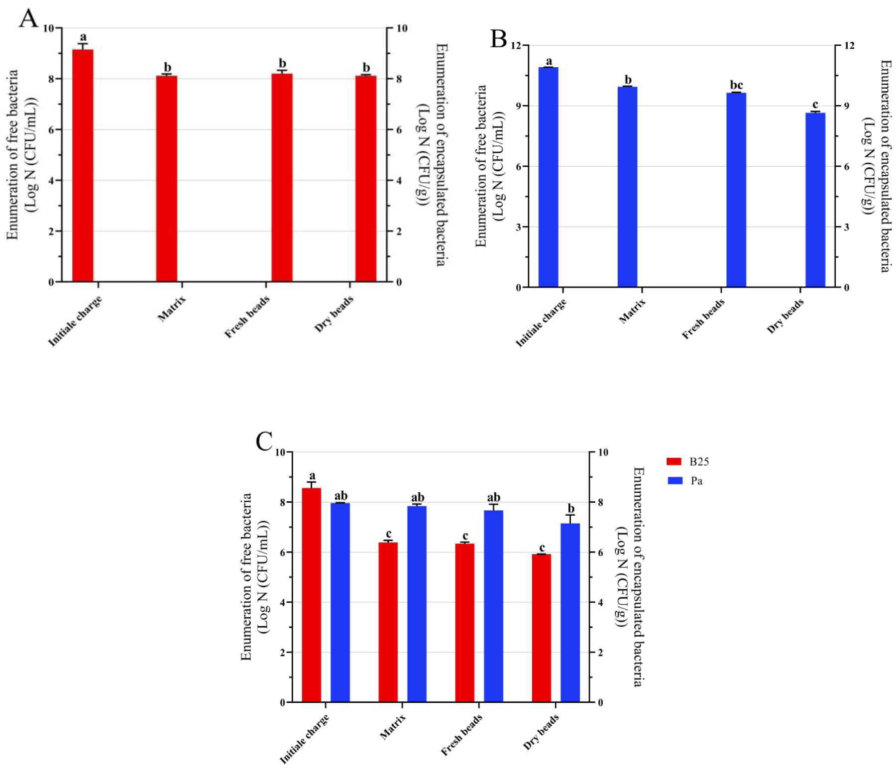
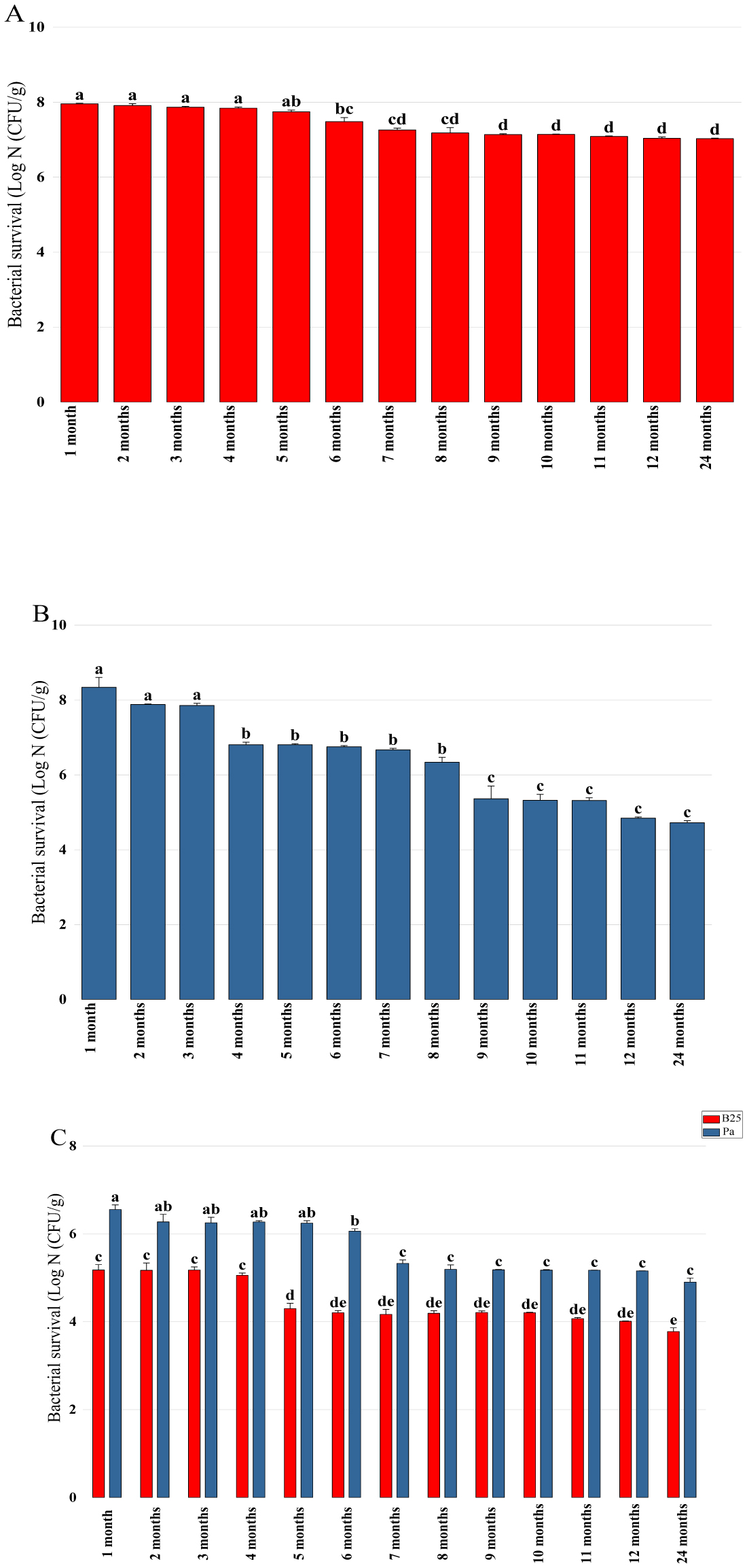
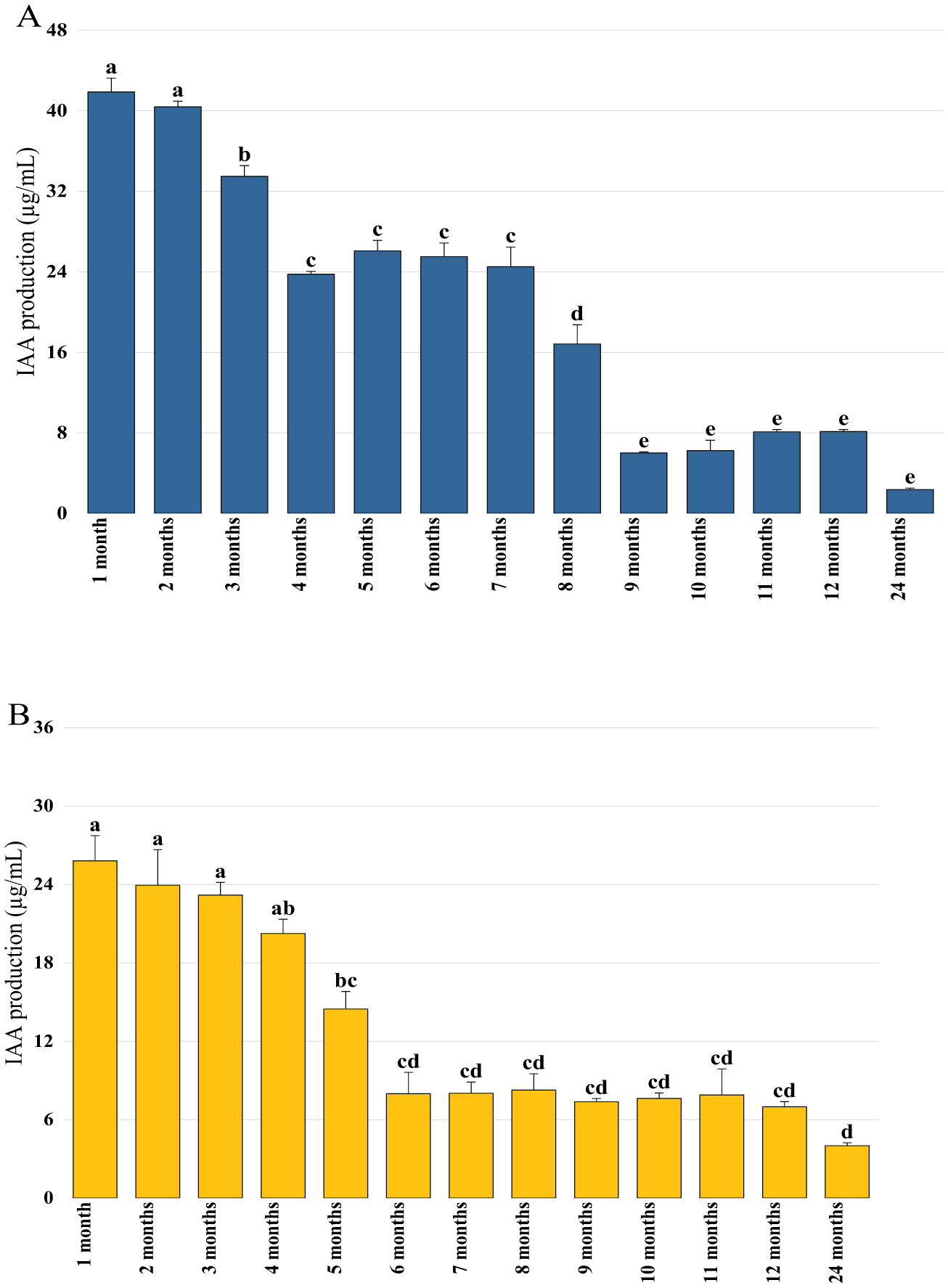
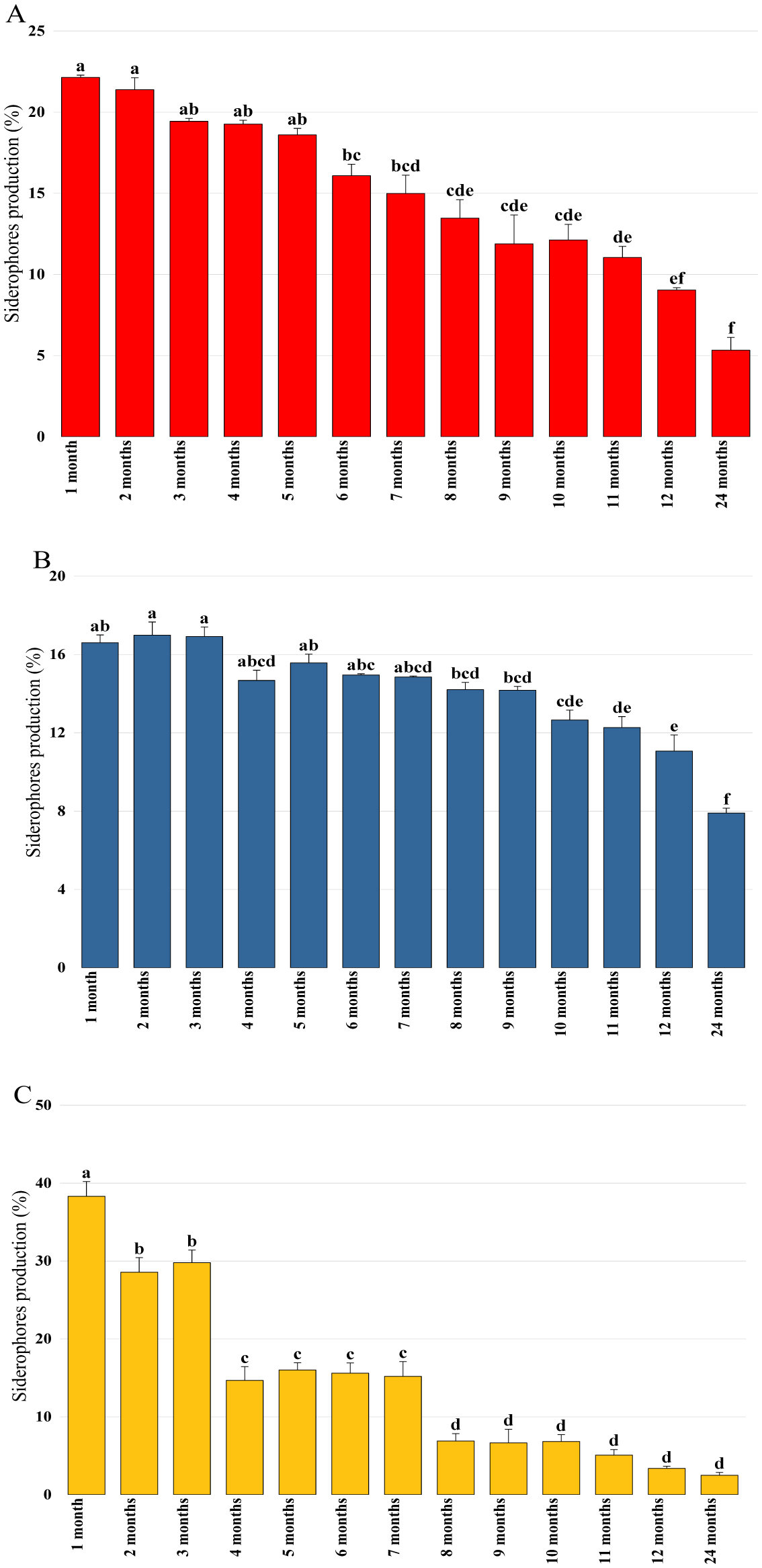
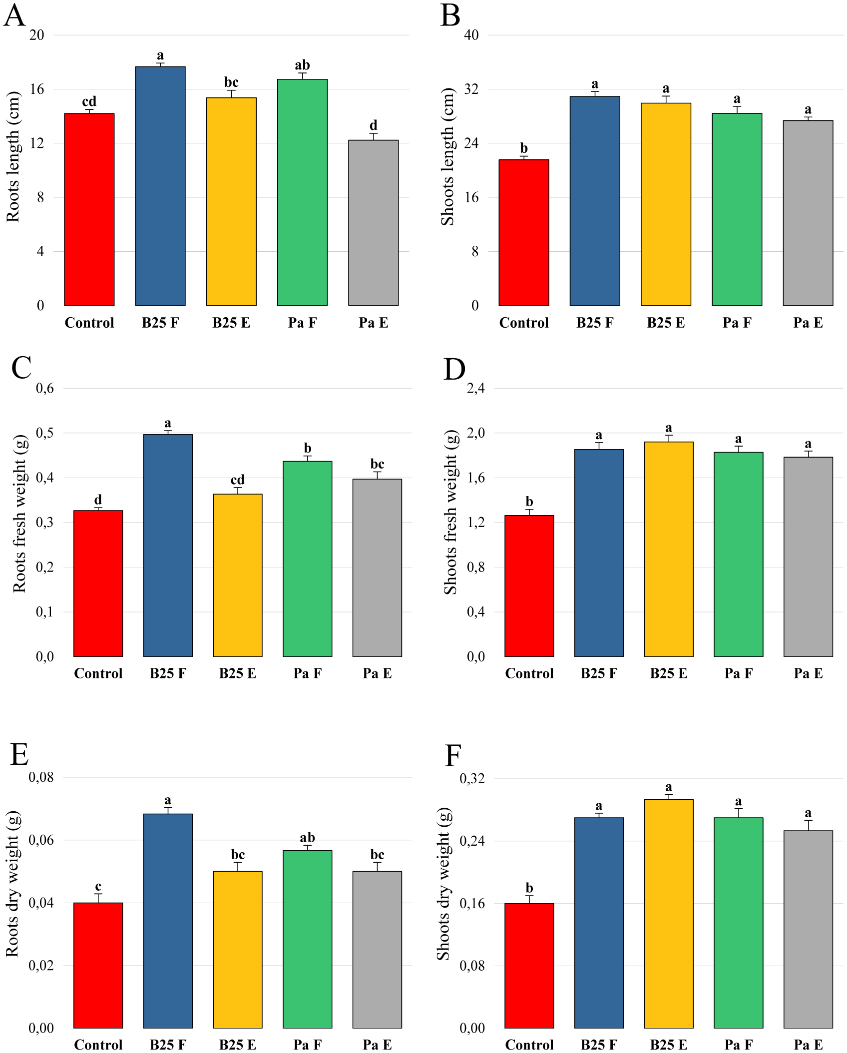
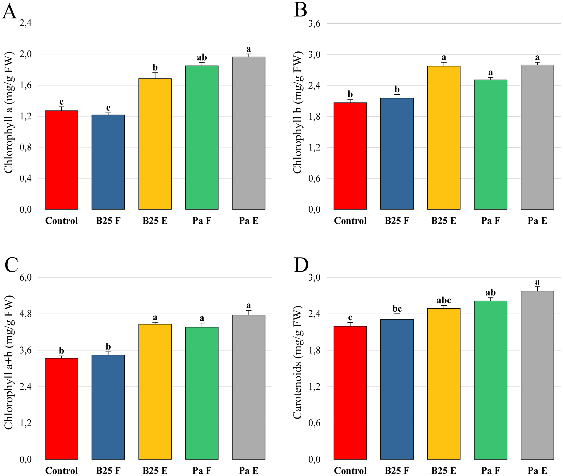
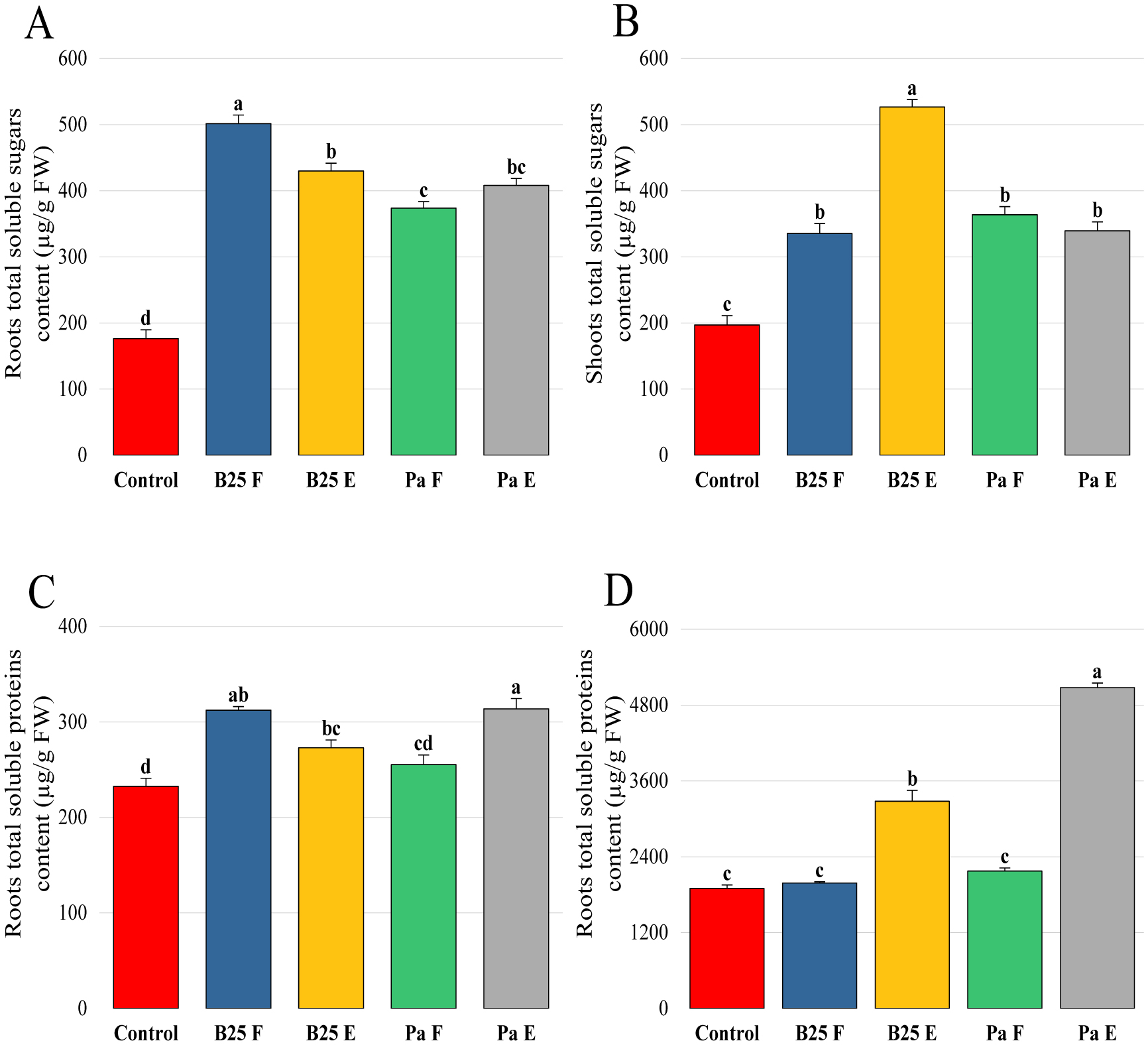
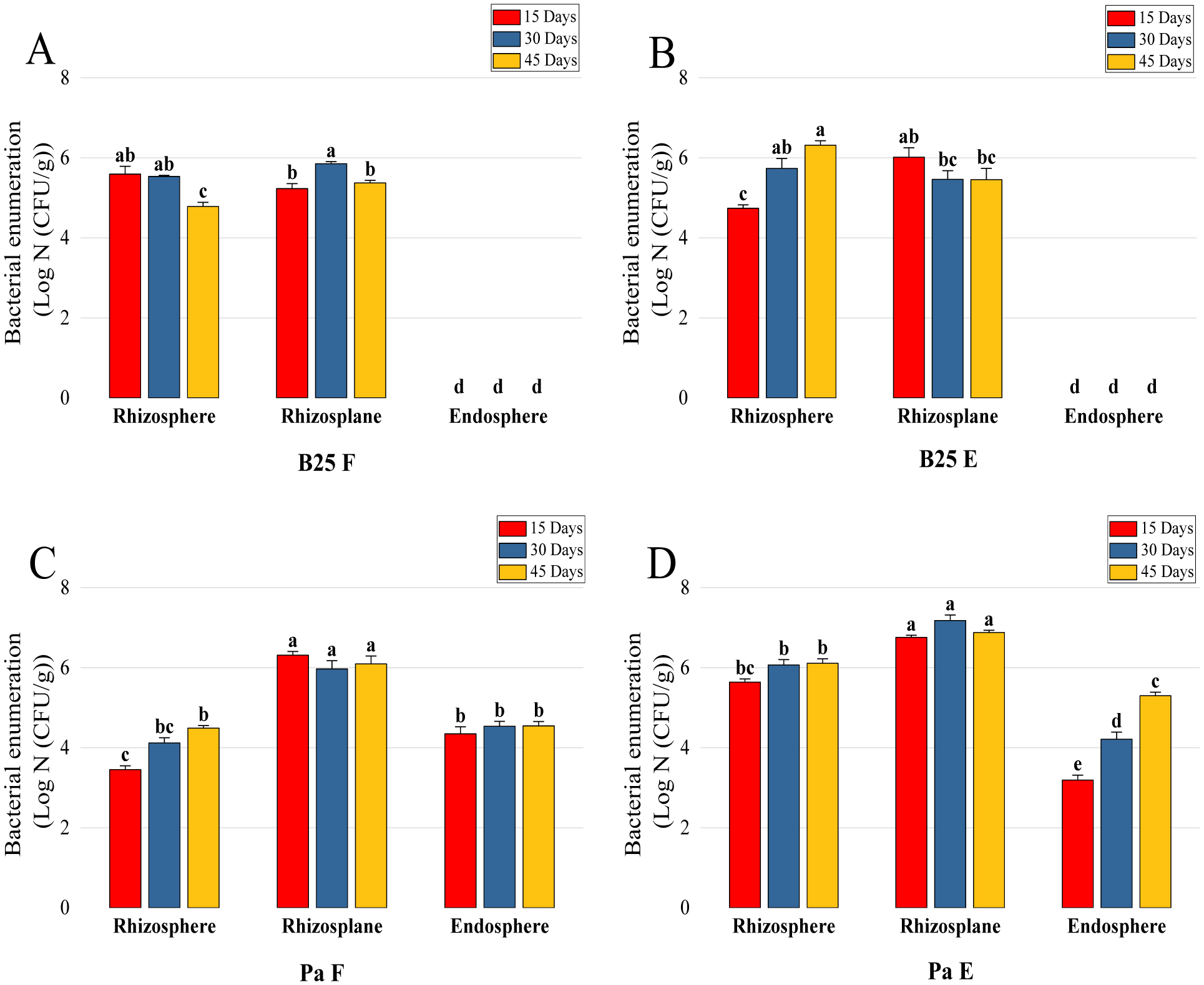
Bioencapsulation in alginate capsules offers an interesting opportunity for the efficient delivery of microbial inoculants for agricultural purposes. The present study evaluated the ionic gelation technique to prepare beads loaded with two plant growth-promoting bacteria (PGPB), Bacillus thuringiensis strain B25 and Pantoea agglomerans strain Pa in 1% alginate supplemented with 5mM proline as an osmoprotectant. Capsule morphology, survival rate, encapsulation efficiency, and viability during 24 months of storage as well as the stability of PGP activities were studied. Our results indicate that more than 99% of bacteria were effectively trapped in the alginate beads, which successfully released live bacteria after 60 days of storage at room temperature. A considerable survival of B. thuringiensis B25 throughout the storage period was detected, while the inoculated concentration of 8.72 × 10⁹ (±0.04 ×10⁹) CFU/mL was reduced to 99.9% for P. agglomerans Pa after 24 months of storage. Notably, a higher survival of individually encapsulated bacteria was observed compared to their co-inoculation. The colonization capacity of model plant Arabidopsis thaliana roots by free and encapsulated bacteria was detected by the triphenyltetrazolium chloride test. Moreover, both strains effectively colonized the rhizosphere, rhizoplane, and endosphere of durum wheat plants and exerted a remarkable improvement in plant growth, estimated as a significant increase in the quantities of total proteins, sugars, and chlorophyll pigments, besides roots and shoots length. This study demonstrated that alginate-encapsulated B. thuringiensis B25 and P. agglomerans Pa could be used as inoculants in agriculture, as their encapsulation ensures robust protection, maintenance of viability and PGP activity, and controlled bacterial biostimulant release into the rhizosphere.
- bioencapsulation,
- sodium alginate,
- PGPB,
- Arabidopsis thaliana,
- durum wheat,
- root colonization
Citation: Amel Balla, Allaoua Silini, Hafsa Cherif-Silini, Francesca Mapelli, Sara Borin. Root colonization dynamics of alginate encapsulated rhizobacteria: implications for Arabidopsis thaliana root growth and durum wheat performance[J]. AIMS Microbiology, 2025, 11(1): 87-125. doi: 10.3934/microbiol.2025006

Related Papers:

Abstract

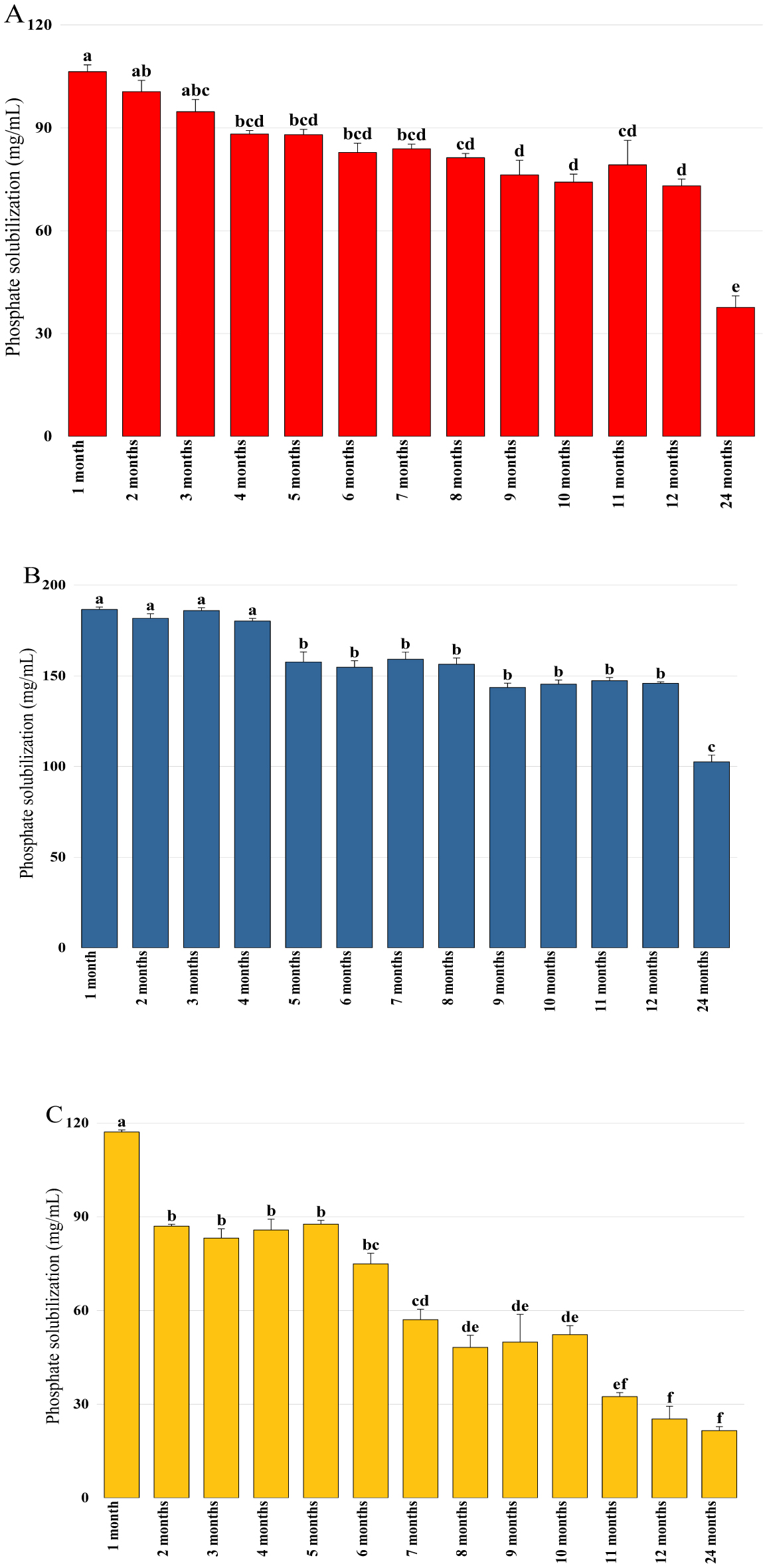
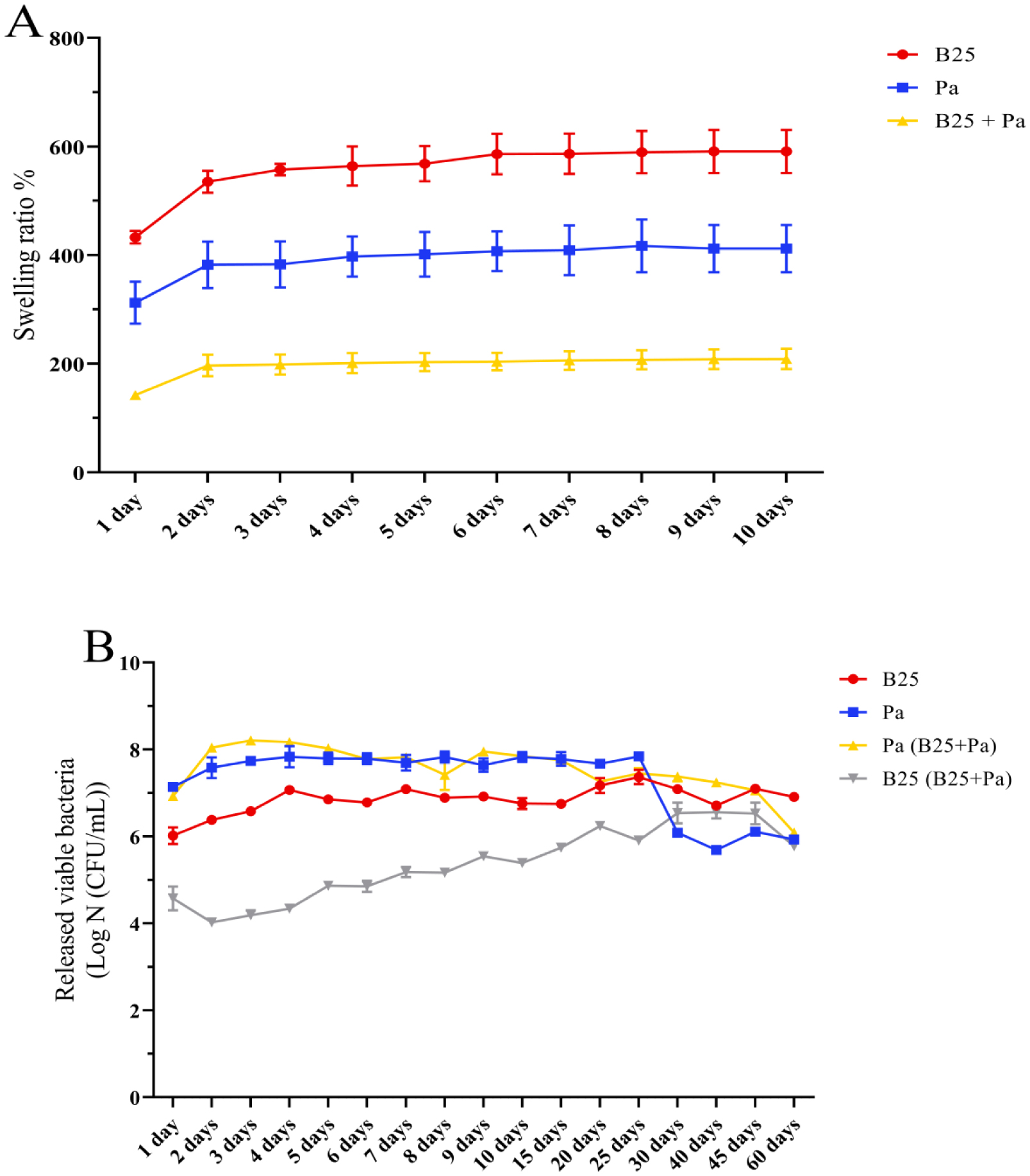
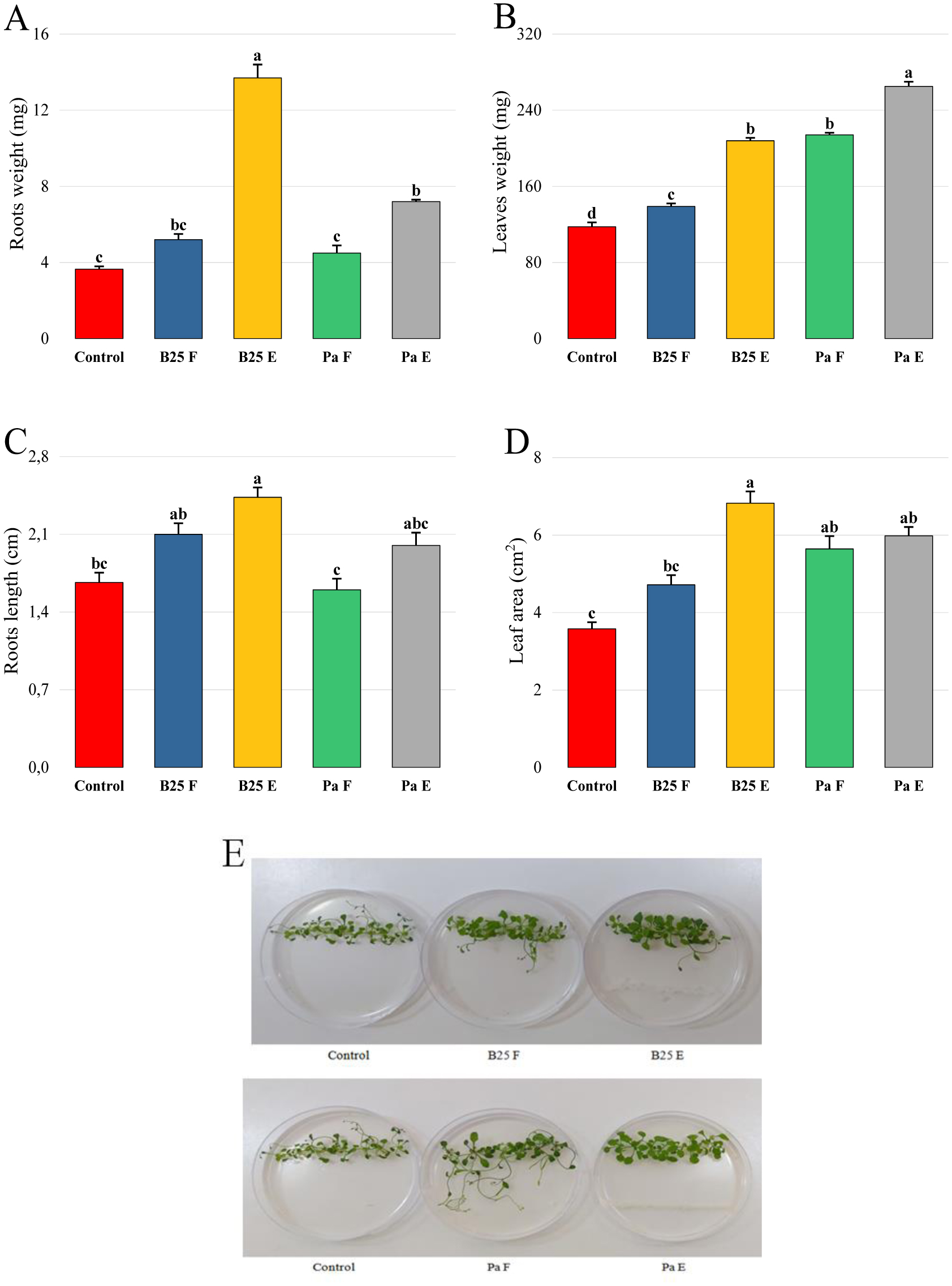
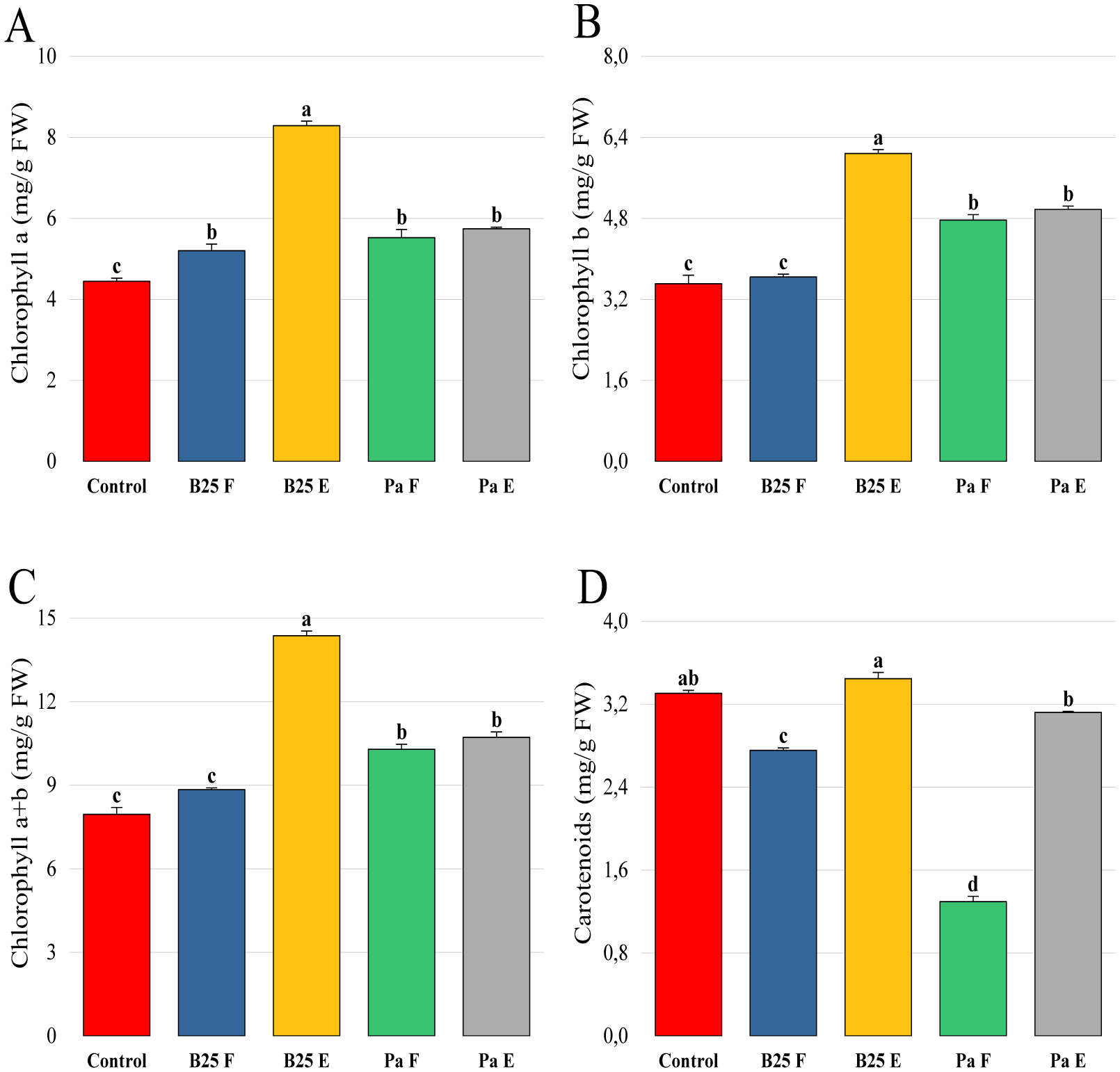
Bioencapsulation in alginate capsules offers an interesting opportunity for the efficient delivery of microbial inoculants for agricultural purposes. The present study evaluated the ionic gelation technique to prepare beads loaded with two plant growth-promoting bacteria (PGPB), Bacillus thuringiensis strain B25 and Pantoea agglomerans strain Pa in 1% alginate supplemented with 5mM proline as an osmoprotectant. Capsule morphology, survival rate, encapsulation efficiency, and viability during 24 months of storage as well as the stability of PGP activities were studied. Our results indicate that more than 99% of bacteria were effectively trapped in the alginate beads, which successfully released live bacteria after 60 days of storage at room temperature. A considerable survival of B. thuringiensis B25 throughout the storage period was detected, while the inoculated concentration of 8.72 × 10⁹ (±0.04 ×10⁹) CFU/mL was reduced to 99.9% for P. agglomerans Pa after 24 months of storage. Notably, a higher survival of individually encapsulated bacteria was observed compared to their co-inoculation. The colonization capacity of model plant Arabidopsis thaliana roots by free and encapsulated bacteria was detected by the triphenyltetrazolium chloride test. Moreover, both strains effectively colonized the rhizosphere, rhizoplane, and endosphere of durum wheat plants and exerted a remarkable improvement in plant growth, estimated as a significant increase in the quantities of total proteins, sugars, and chlorophyll pigments, besides roots and shoots length. This study demonstrated that alginate-encapsulated B. thuringiensis B25 and P. agglomerans Pa could be used as inoculants in agriculture, as their encapsulation ensures robust protection, maintenance of viability and PGP activity, and controlled bacterial biostimulant release into the rhizosphere.

Conflict of interest

The authors declare no conflicts of interest.

Author contributions

Conceptualization, A.B., HCS.,and A.S.; methodology, A.S., and H.C-S.; software, A.B.; validation, A.S., HCS., F.M. and S.B.; formal analysis, F.M., and S.B.; investigation, A.B., and F.M.; data curation, A.B., and A.S.; writing—original draft preparation, A.B.; writing—review and editing, A.S., HCS., F.M., and S.B.; visualization, A.B.; supervision, A.S., and H.C-S.; All authors have read and agreed to the published version of the manuscript.

Funding

This research received no external funding.

References

[1]	Ehrlich PR, Harte J (2015) To feed the world in 2050 will require a global revolution. Proc Natl Acad Sci 112: 14743-14744. https://doi.org/10.1073/pnas.1519841112
[2]	Ali M, Cybulska J, Frąc M, et al. (2023) Application of polysaccharides for the encapsulation of beneficial microorganisms for agricultural purposes: A review. Int J Biol Macromol 125366. https://doi.org/10.1016/j.ijbiomac.2023.125366
[3]	FAO.Pesticides use, pesticides trade and pesticides indicators. Global, regional and country trends, 1990–2019. FAOSTAT Anal Brief Ser No 29 Rome (2021) .
[4]	Rani L, Thapa K, Kanojia N, et al. (2021) An extensive review on the consequences of chemical pesticides on human health and environment. J Cleaner Prod 283: 124657. https://doi.org/10.1016/j.jclepro.2020.124657
[5]	Intisar A, Ramzan A, Sawaira T, et al. (2022) Occurrence, toxic effects, and mitigation of pesticides as emerging environmental pollutants using robust nanomaterials–A review. Chemosphere 293: 133538. https://doi.org/10.1016/j.chemosphere.2022.133538
[6]	Sharma N, Singhvi R (2017) Effects of chemical fertilizers and pesticides on human health and environment: a review. Int J Agric Environ Biotechnol 10: 675-680. https://doi.org/10.5958/2230-732X.2017.00083.3
[7]	Kaur R, Kaur S (2018) Biological alternates to synthetic fertilizers: efficiency and future scopes. Indian J Agric Res 52: 587-595. https://doi.org/10.18805/IJARe.A-5117
[8]	Hossain MA, Hossain MS, Akter M (2023) Challenges faced by plant growth-promoting bacteria in field-level applications and suggestions to overcome the barriers. Physiol Mol Plant Pathol 102029. https://doi.org/10.1016/j.pmpp.2023.102029
[9]	Singh K, Guleria V, Kaushal S (2023) Utilization of Biofertilizers and plant growth promoters in hydroponic production system. Curr J Appl Sci Technol 42: 13-23. https://doi.org/10.9734/cjast/2023/v42i374243
[10]	Orozco-Mosqueda MDC, Santoyo G, Glick BR (2023) Recent advances in the bacterial phytohormone modulation of plant growth. Plants 12: 606. https://doi.org/10.3390/plants12030606
[11]	Etesami H, Jeong BR, Glick BR (2023) Biocontrol of plant diseases by Bacillus spp. Physiol Mol Plant Pathol 102048. https://doi.org/10.1016/j.pmpp.2023.102048
[12]	Remus R, Ruppel S, Jacob HJ, et al. (2000) Colonization behaviour of two enterobacterial strains on cereals. Biol Fertil Soils 30: 550-557. https://doi.org/10.1007/s003740050035
[13]	Mishra A, Chauhan PS, Chaudhry V, et al. (2011) Rhizosphere competent Pantoea agglomerans enhances maize (Zea mays) and chickpea (Cicer arietinum L.) growth, without altering the rhizosphere functional diversity. Antonie Van Leeuwenhoek 100: 405-413. https://doi.org/10.1007/s10482-011-9596-8
[14]	Cherif-Silini H, Thissera B, Bouket AC, et al. (2019) Durum wheat stress tolerance induced by endophyte Pantoea agglomerans with genes contributing to plant functions and secondary metabolite arsenal. Int J Mol Sci 20: 3989. https://doi.org/10.3390/ijms20163989
[15]	Lorenzi AS, Bonatelli ML, Chia MA, et al. (2022) Opposite sides of Pantoea agglomerans and its associated commercial outlook. Microorganisms 10: 2072. https://doi.org/10.3390/microorganisms10102072
[16]	Torres AR, Araújo WL, Cursino L, et al. (2013) Colonization of Madagascar periwinkle (Catharanthus roseus), by endophytes encoding gfp marker. Arch Microbiol 195: 483-489. https://doi.org/10.1007/s00203-013-0897-3
[17]	Herrera SD, Grossi C, Zawoznik M, et al. (2016) Wheat seeds harbour bacterial endophytes with potential as plant growth promoters and biocontrol agents of Fusarium graminearum. Microbiol Res 186: 37-43. https://doi.org/10.1016/j.micres.2016.03.002
[18]	Gomis-Cebolla J, Berry C (2023) Bacillus thuringiensis as a biofertilizer in crops and their implications in the control of phytopathogens and insect pests. Pest Manage Sci 79: 2992-3001. https://doi.org/10.1002/ps.7560
[19]	Azizoglu U (2019) Bacillus thuringiensis as a biofertilizer and biostimulator: a mini-review of the little-known plant growth-promoting properties of Bt. Curr Microbiol 76: 1379-1385. https://doi.org/10.1007/s00284-019-01705-9
[20]	Mącik M, Gryta A, Frąc M (2020) Biofertilizers in agriculture: An overview on concepts, strategies and effects on soil microorganisms. Adv Agron 162: 31-87. https://doi.org/10.1016/bs.agron.2020.02.001
[21]	Rai S, Mago Y, Aggarwal G, et al. (2023) Liquid bioformulation: a trending approach towards achieving sustainable agriculture. Mol Biotechnol 1–26. https://doi.org/10.1007/s12033-023-00901-0
[22]	Balla A, Silini A, Cherif-Silini H, et al. (2022) Recent advances in encapsulation techniques of plant growth-promoting microorganisms and their prospects in the sustainable agriculture. Appl Sci 12: 9020. https://doi.org/10.3390/app12189020
[23]	Song S, Liu Y, Wang NR, et al. (2021) Mechanisms in plant–microbiome interactions: lessons from model systems. Curr Opin Plant Biol 62: 102003. https://doi.org/10.1016/j.pbi.2021.102003
[24]	Grosse-Heilmann M, Cristiano E, Deidda R, et al. (2024) Durum wheat productivity today and tomorrow: A review of influencing factors and climate change effects. Resour Environ Sustainability 100170. https://doi.org/10.1016/j.resenv.2024.100170
[25]	Saadaoui N, Silini A, Cherif-Silini H, et al. (2022) Semi-arid-habitat-adapted plant-growth-promoting rhizobacteria allows efficient wheat growth promotion. Agronomy 12: 2221. https://doi.org/10.3390/agronomy12092221
[26]	Wu Z, Zhao Y, Kaleem I, et al. (2011) Preparation of calcium–alginate microcapsuled microbial fertilizer coating Klebsiella oxytoca Rs-5 and its performance under salinity stress. Eur J Soil Biol 47: 152-159. https://doi.org/10.1016/j.ejsobi.2010.11.008
[27]	Panichikkal J, Prathap G, Nair RA, et al. (2021) Evaluation of plant probiotic performance of Pseudomonas sp. encapsulated in alginate supplemented with salicylic acid and zinc oxide nanoparticles. Int J Biol Macromol 166: 138-143. https://doi.org/10.1016/j.ijbiomac.2020.10.110
[28]	Chi Y, Wang D, Jiang M, et al. (2020) Microencapsulation of Bacillus megaterium NCT-2 and its effect on remediation of secondary salinization soil. J Microencapsulation 37: 134-143. https://doi.org/10.1080/02652048.2019.1705409
[29]	Kerbab S, Silini A, Chenari Bouket A, et al. (2021) Mitigation of NaCl stress in wheat by rhizosphere engineering using salt habitat adapted PGPR halotolerant bacteria. Appl Sci 11: 1034. https://doi.org/10.3390/app11031034
[30]	Saidi S, Cherif-Silini H, Chenari Bouket A, et al. (2021) Improvement of Medicago sativa crops productivity by the co-inoculation of Sinorhizobium meliloti–actinobacteria under salt stress. Curr Microbiol 78: 1344-1357. https://doi.org/10.1007/s00284-021-02394-z
[31]	Slama HB, Cherif-Silini H, Chenari Bouket A, et al. (2019) Screening for Fusarium antagonistic bacteria from contrasting niches designated the endophyte Bacillus halotolerans as plant warden against Fusarium. Front Microbiol 9: 3236. https://doi.org/10.3389/fmicb.2018.03236
[32]	Tsavkelova EA, Cherdyntseva TA, Netrusov AI (2004) Bacteria associated with the roots of epiphytic orchids. Microbiology 73: 710-715. https://doi.org/10.1007/s11021-005-0013-z
[33]	Silini A, Cherif-Silini H, Yahiaoui B (2016) Growing varieties durum wheat (Triticum durum) in response to the effect of osmolytes and inoculation by Azotobacter chroococcum under salt stress. Afr J Microbiol Res 10: 387-399. https://doi.org/10.5897/AJMR2015.7723
[34]	DuBois M, Gilles KA, Hamilton JK, et al. (1956) Colorimetric method for determination of sugars and related substances. Anal Chem 28: 350-356. https://doi.org/10.1021/ac60111a017
[35]	Lowry OH, Rosebrough NJ, Farr AL, et al. (1951) Protein measurement with the Folin phenol reagent. J Biol Chem 193: 265-275. https://doi.org/10.1016/S0021-9258(19)52451-6
[36]	Berninger T, González López Ó, Bejarano A, et al. (2018) Maintenance and assessment of cell viability in formulation of non-sporulating bacterial inoculants. Microb Biotechnol 11: 277-301. https://doi.org/10.1111/1751-7915.12880
[37]	Daffonchio D, Hirt H, Berg G (2015) Plant-microbe interactions and water management in arid and saline soils. Principles of Plant-Microbe Interactions: Microbes for Sustainable Agriculture . Cham: Springer 265-276. https://doi.org/10.1007/978-3-319-08575-3_28
[38]	Hayat S, Hayat Q, Alyemeni MN, et al. (2012) Role of proline under changing environments: a review. Plant Signaling Behav 7: 1456-1466. https://doi.org/10.4161/psb.21949
[39]	Wu Z, Li X, Liu X, et al. (2020) Membrane shell permeability of Rs-198 microcapsules and their ability for growth promoting bioactivity compound releasing. RSC Adv 10: 1159-1171. https://doi.org/10.1039/C9RA06935F
[40]	Kaur R, Kaur S, Dwibedi V, et al. (2023) Development and characterization of rice bran-gum Arabic based encapsulated biofertilizer for enhanced shelf life and controlled bacterial release. Front Microbiol 14: 1267730. https://doi.org/10.3389/fmicb.2023.1267730
[41]	García AH (2011) Anhydrobiosis in bacteria: from physiology to applications. J Biosci 36: 939-950. https://doi.org/10.1007/s12038-011-9107-0
[42]	Schoebitz M, Simonin H, Poncelet D (2012) Starch filler and osmoprotectants improve the survival of rhizobacteria in dried alginate beads. J Microencapsulation 29: 532-538. https://doi.org/10.3109/02652048.2012.665090
[43]	Liffourrena AS, Lucchesi GI (2018) Alginate-perlite encapsulated Pseudomonas putida A (ATCC 12633) cells: Preparation, characterization and potential use as plant inoculants. J Biotechnol 278: 28-33. https://doi.org/10.1016/j.jbiotec.2018.04.019
[44]	Timmusk S, Behers L, Muthoni J, et al. (2017) Perspectives and challenges of microbial application for crop improvement. Front Plant Sci 8: 49. https://doi.org/10.3389/fpls.2017.00049
[45]	Guo L, Wu Z, Rasool A, et al. (2012) Effects of free and encapsulated co-culture bacteria on cotton growth and soil bacterial communities. Eur J Soil Biol 53: 16-22. https://doi.org/10.1016/j.ejsobi.2012.08.003
[46]	Anwar MS, Paliwal A, Firdous N, et al. (2019) Co-culture development and bioformulation efficacy of psychrotrophic PGPRs to promote growth and development of pea (Pisum sativum) plant. J Gen Appl Microbiol 65: 88-95. https://doi.org/10.2323/jgam.2018.05.007
[47]	Santos MS, Nogueira MA, Hungria M (2019) Microbial inoculants: reviewing the past, discussing the present and previewing an outstanding future for the use of beneficial bacteria in agriculture. Amb Express 9: 1-22. https://doi.org/10.1186/s13568-019-0932-0
[48]	Ozdal M, Ozdal OG, Sezen A, et al. (2017) Continuous production of indole-3-acetic acid by immobilized cells of Arthrobacter agilis. 3 Biotech 7: 1-6. https://doi.org/10.1007/s13205-017-0605-0
[49]	Sandhya VZAS, SK ZA, Grover M, et al. (2009) Alleviation of drought stress effects in sunflower seedlings by the exopolysaccharides producing Pseudomonas putida strain GAP-P45. Biol Fertil Soils 46: 17-26. https://doi.org/10.1007/s00374-009-0401-z
[50]	Duca DR, Glick BR (2020) Indole-3-acetic acid biosynthesis and its regulation in plant-associated bacteria. Appl Microbiol Biotechnol 104: 8607-8619. https://doi.org/10.1007/s00253-020-10869-5
[51]	Höper D, Bernhardt J, Hecker M (2006) Salt stress adaptation of Bacillus subtilis: a physiological proteomics approach. Proteomics 6: 1550-1562. https://doi.org/10.1002/pmic.200500197
[52]	Dunyashev TP, Laptev GY, Yildirim EA, et al. (2021) Identification of genes associated with the synthesis of siderophores by the Bacillus subtilis. J Livestock Sci 12: 287-291. https://doi.org/10.33259/JLivestSci.2021.287-291
[53]	Yadav AN, Kumar V, Dhaliwal HS, et al. (2018) Microbiome in crops: diversity, distribution, and potential role in crop improvement. Crop improvement through microbial biotechnology . Elsevier 305-332. https://doi.org/10.1016/B978-0-444-63987-5.00015-3
[54]	Pan L, Cai B (2023) Phosphate-solubilizing bacteria: advances in their physiology, molecular mechanisms and microbial community effects. Microorganisms 11: 2904. https://doi.org/10.3390/microorganisms11122904
[55]	Wang JJ, Yan AH, Wang W, et al. (2016) Screening, identification and phosphate-solubilizing characteristics of phosphate-solubilizing bacteria strain D2 (Pantoea sp.) in rhizosphere of Pinus tabuliformis in iron tailings yard. Ying Yong Sheng tai xue bao=The Journal of Applied Ecology 27: 3705-3711.
[56]	Kalayu G (2019) Phosphate solubilizing microorganisms: promising approach as biofertilizers. Int J Agron 4917256. https://doi.org/10.1155/2019/4917256
[57]	Khourchi S, Elhaissoufi W, Loum M, et al. (2022) Phosphate solubilizing bacteria can significantly contribute to enhance P availability from polyphosphates and their use efficiency in wheat. Microbiol Res 262: 127094. https://doi.org/10.1016/j.micres.2022.127094
[58]	Suleimanova AD, Beinhauer A, Valeeva LR, et al. (2015) Novel glucose-1-phosphatase with high phytase activity and unusual metal ion activation from soil bacterium Pantoea sp. strain 3.5. 1. Appl Environ Microbiol 81: 6790-6799. https://doi.org/10.1128/AEM.01384-15
[59]	Park JH, Lee HH, Han CH, et al. (2016) Synergistic effect of co-inoculation with phosphate-solubilizing bacteria. Korean J Agric Sci 43: 401-414. https://doi.org/10.7744/kjoas.20160043
[60]	Tu L, He Y, Shan C, et al. (2016) Preparation of microencapsulated Bacillus subtilis SL-13 seed coating agents and their effects on the growth of cotton seedlings. BioMed Res Int 16. https://doi.org/10.1155/2016/3251357
[61]	Liu B, Luo J, Wang X, et al. (2013) Alginate/quaternized carboxymethyl chitosan/clay nanocomposite microspheres: preparation and drug-controlled release behavior. J Biomater Sci Polym Ed 4: 589-605. https://doi.org/10.1080/09205063.2012.701160
[62]	He Y, Wu Z, Tu L, et al. (2015) Encapsulation and characterization of slow-release microbial fertilizer from the composites of bentonite and alginate. Appl Clay Sci 109: 68-75. https://doi.org/10.1016/j.clay.2015.02.001
[63]	Pour MM, Saberi-Riseh R, Mohammadinejad R, et al. (2019) Investigating the formulation of alginate-gelatin encapsulated Pseudomonas fluorescens (VUPF5 and T17-4 strains) for controlling Fusarium solani on potato. Int J Biol Macromol 133: 603-613. https://doi.org/10.1016/j.ijbiomac.2019.04.071
[64]	Al-Qaysi SA, Al-Haideri H, Al-Shimmary SM, et al. (2021) Bioactive levan-Type exopolysaccharide produced by Pantoea agglomerans ZMR7: Characterization and optimization for enhanced production. J Microbiol Biotechnol 31: 696. https://doi.org/10.4014/jmb.2101.01025
[65]	Wang M, Geng L, Xue B, et al. (2021) Structure characteristics and function of a novel extracellular polysaccharide from Bacillus thuringiensis strain 4D19. Int J Biol Macromol 189: 956-964. https://doi.org/10.1016/j.ijbiomac.2021.08.193
[66]	Donati I, Holtan S, Mørch YA, et al. (2005) New hypothesis on the role of alternating sequences in calcium– alginate gels. Biomacromolecules 6: 1031-1040. https://doi.org/10.1021/bm049306e
[67]	Liew CV, Chan LW, Ching AL, et al. (2006) Evaluation of sodium alginate as drug release modifier in matrix tablets. Int J Pharm 309: 25-37. https://doi.org/10.1016/j.ijpharm.2005.10.040
[68]	Allard-Massicotte R, Tessier L, Lécuyer F, et al. (2016) Bacillus subtilis early colonization of Arabidopsis thaliana roots involves multiple chemotaxis receptors. MBio 7: 10-1128. https://doi.org/10.1128/mBio.01664-16
[69]	Doornbos RF, Geraats BP, Kuramae EE, et al. (2011) Effects of jasmonic acid, ethylene, and salicylic acid signaling on the rhizosphere bacterial community of Arabidopsis thaliana. Mol Plant Microbe Interact 24: 395-407. https://doi.org/10.1094/MPMI-05-10-0115
[70]	Polisetti S, Bible AN, Morrell-Falvey JL, et al. (2016) Raman chemical imaging of the rhizosphere bacterium Pantoea sp. YR343 and its co-culture with Arabidopsis thaliana. Analyst 141: 2175-2182. https://doi.org/10.1039/C6AN00080K
[71]	Beauregard PB, Chai Y, Vlamakis H, et al. (2013) Bacillus subtilis biofilm induction by plant polysaccharides. Proce Natl Acad Sci 110: 1621-1630. https://doi.org/10.1073/pnas.1218984110
[72]	Fan D, Subramanian S, Smith DL (2020) Plant endophytes promote growth and alleviate salt stress in Arabidopsis thaliana. Sci Rep 10: 12740. https://doi.org/10.1038/s41598-020-69713-5
[73]	Graça AT, Hall M, Persson K, et al. (2021) High-resolution model of Arabidopsis photosystem II reveals the structural consequences of digitonin-extraction. Sci Rep 11: 15534. https://doi.org/10.1038/s41598-021-94914-x
[74]	Mirskaya GV, Khomyakov YV, Rushina NA, et al. (2022) Plant development of early-maturing spring wheat (Triticum aestivum L.) under inoculation with Bacillus sp. V2026. Plants 11: 1817. https://doi.org/10.3390/plants11141817
[75]	Sood G, Kaushal R, Sharma M (2020) Significance of inoculation with Bacillus subtilis to alleviate drought stress in wheat (Triticum aestivum L.). Vegetos 33: 782-792. https://doi.org/10.1007/s42535-020-00149-y
[76]	Rojas-Padilla J, de-Bashan LE, Parra-Cota FI, et al. (2022) Microencapsulation of Bacillus Strains for Improving Wheat (Triticum turgidum Subsp. durum) Growth and Development. Plants 11: 2920. https://doi.org/10.3390/plants11212920
[77]	Suman A, Shukla L, Marag PS, et al. (2020) Potential use of plant colonizing Pantoea as generic plant growth promoting bacteria for cereal crops. J Environ Biol 41: 987-994. https://doi.org/10.22438/jeb/41/5/MRN-1250
[78]	Hussain A, Hasnain S (2011) Interactions of bacterial cytokinins and IAA in the rhizosphere may alter phytostimulatory efficiency of rhizobacteria. World J Microbiol Biotechnol 27: 2645-2654. https://doi.org/10.1007/s11274-011-0738-y
[79]	Yaghoubi Khanghahi M, Leoni B, Crecchio C (2021) Photosynthetic responses of durum wheat to chemical/microbiological fertilization management under salt and drought stresses. Acta Physiol Plant 43: 1-14. https://doi.org/10.1007/s11738-021-03289-z
[80]	Yong JWH, Ng YF, Tan SN, et al. (2010) Effect of fertilizer application on photosynthesis and oil yield of jatropha curcas L. Photosynthetica 48: 208-218. https://doi.org/10.1007/s11099-010-0026-3
[81]	Kanagendran A, Chatterjee P, Liu B, et al. (2019) Foliage inoculation by Burkholderia vietnamiensis CBMB40 antagonizes methyl jasmonate-mediated stress in Eucalyptus grandis. J Plant Physiol 242: 153032. https://doi.org/10.1016/j.jplph.2019.153032
[82]	Acosta-Motos JR, Ortuño MF, Bernal-Vicente A, et al. (2017) Plant responses to salt stress: adaptive mechanisms. Agronomy 7: 18. https://doi.org/10.3390/agronomy7010018
[83]	Singh BK, Trivedi P, Egidi E, et al. (2020) Crop microbiome and sustainable agriculture. Nat Rev Microbiol 18: 601-602. https://doi.org/10.1038/s41579-020-00446-y
[84]	Bhise KK, Dandge PB (2019) Alleviation of salinity stress in rice plant by encapsulated salt tolerant plant growth promoting bacteria Pantoea agglomerans strain KL and its root colonization ability. Arch Agron Soil Sci 65: 1955-1968. https://doi.org/10.1080/03650340.2019.1584395
[85]	He Y, Wu Z, Ye BC, et al. (2016) Viability evaluation of alginate-encapsulated Pseudomonas putida Rs-198 under simulated salt-stress conditions and its effect on cotton growth. Eur J Soil Biol 75: 135-141. https://doi.org/10.1016/j.ejsobi.2016.05.002
[86]	Soluch R, Hülter NF, Romero Picazo D, et al. (2021) Colonization dynamics of Pantoea agglomerans in the wheat root habitat. Environ Microbiol 23: 2260-2273. https://doi.org/10.1111/1462-2920.15430
[87]	Compant S, Clément C, Sessitsch A (2010) Plant growth-promoting bacteria in the rhizo-and endosphere of plants: their role, colonization, mechanisms involved and prospects for utilization. Soil Biol Biochem 42: 669-678. https://doi.org/10.1016/j.soilbio.2009.11.024
[88]	Kumar A, Prakash A, Johri BN (2011) Bacillus as PGPR in crop ecosystem. Bacteria in agrobiology: crop ecosystems . Berlin Heidelberg: Springer 37-59. https://doi.org/10.1007/978-3-642-18357-7_2

microbiol-11-01-006-s001.pdf

Reader Comments

Your name:*

Email:*
© 2025 the Author(s), licensee AIMS Press. This is an open access article distributed under the terms of the Creative Commons Attribution License (http://creativecommons.org/licenses/by/4.0)