Individual-based and continuum models of phenotypically heterogeneous growing cell populations

Fiona R Macfarlane; Xinran Ruan; Tommaso Lorenzi; Fiona R Macfarlane; Xinran Ruan; Tommaso Lorenzi

doi:10.3934/bioeng.2022007

AIMS Bioengineering

2022, Volume 9, Issue 1: 68-92. doi: 10.3934/bioeng.2022007

Previous Article Next Article

Research article Special Issues

Individual-based and continuum models of phenotypically heterogeneous growing cell populations

1.
School of Mathematics and Statistics, University of St Andrews, United Kingdom
2.
School of Mathematical Sciences, Capital Normal University, 100048 Beijing, P.R. China
3.
Department of Mathematical Sciences “G. L. Lagrange”, Politecnico di Torino, 10129 Torino, Italy

Received: 13 February 2022 Revised: 10 March 2022 Accepted: 16 March 2022 Published: 18 March 2022

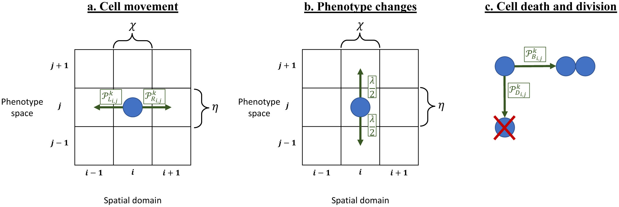
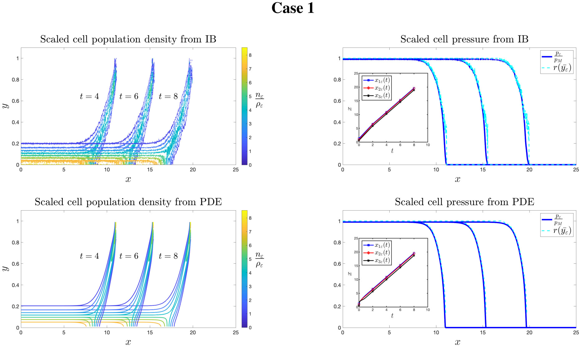
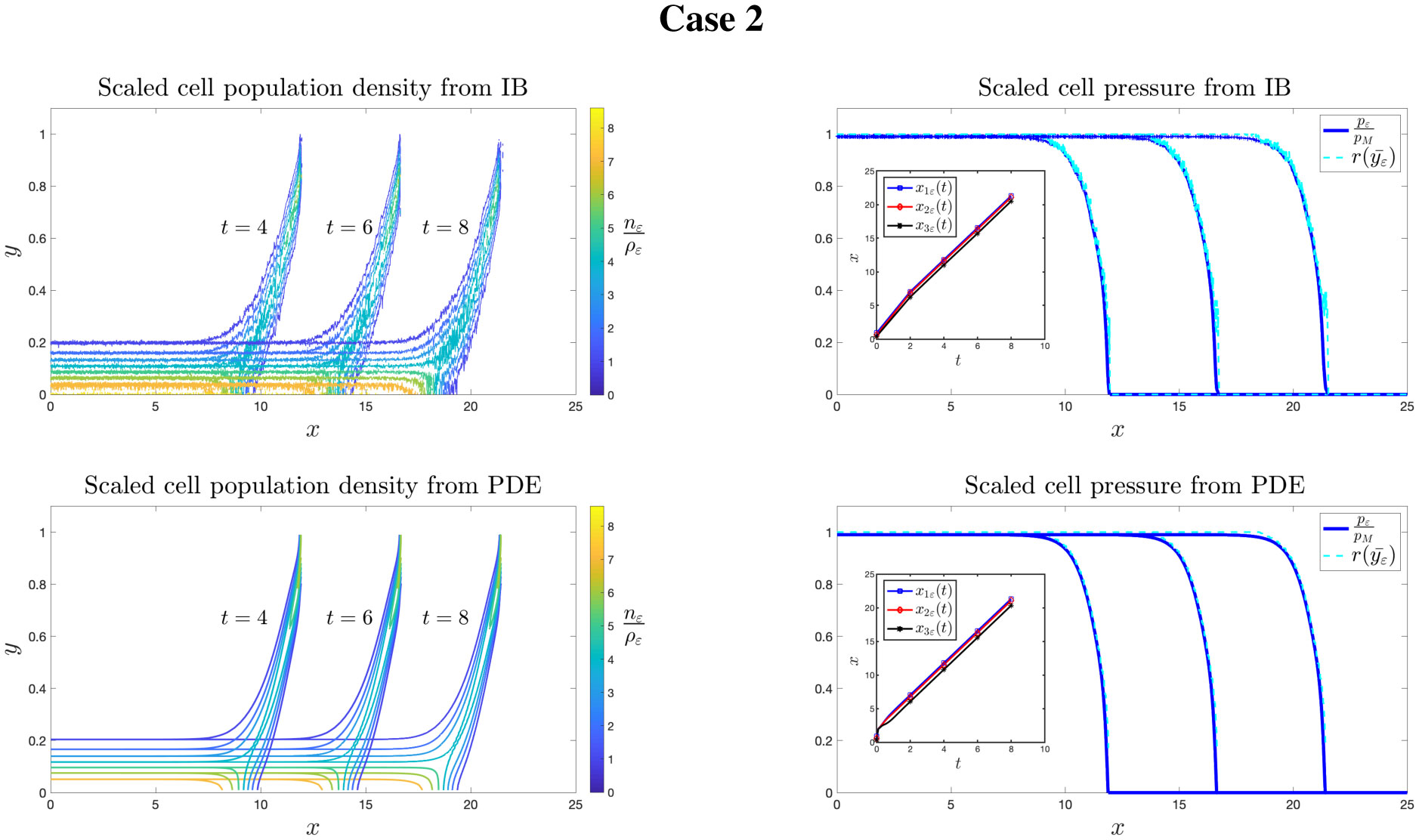
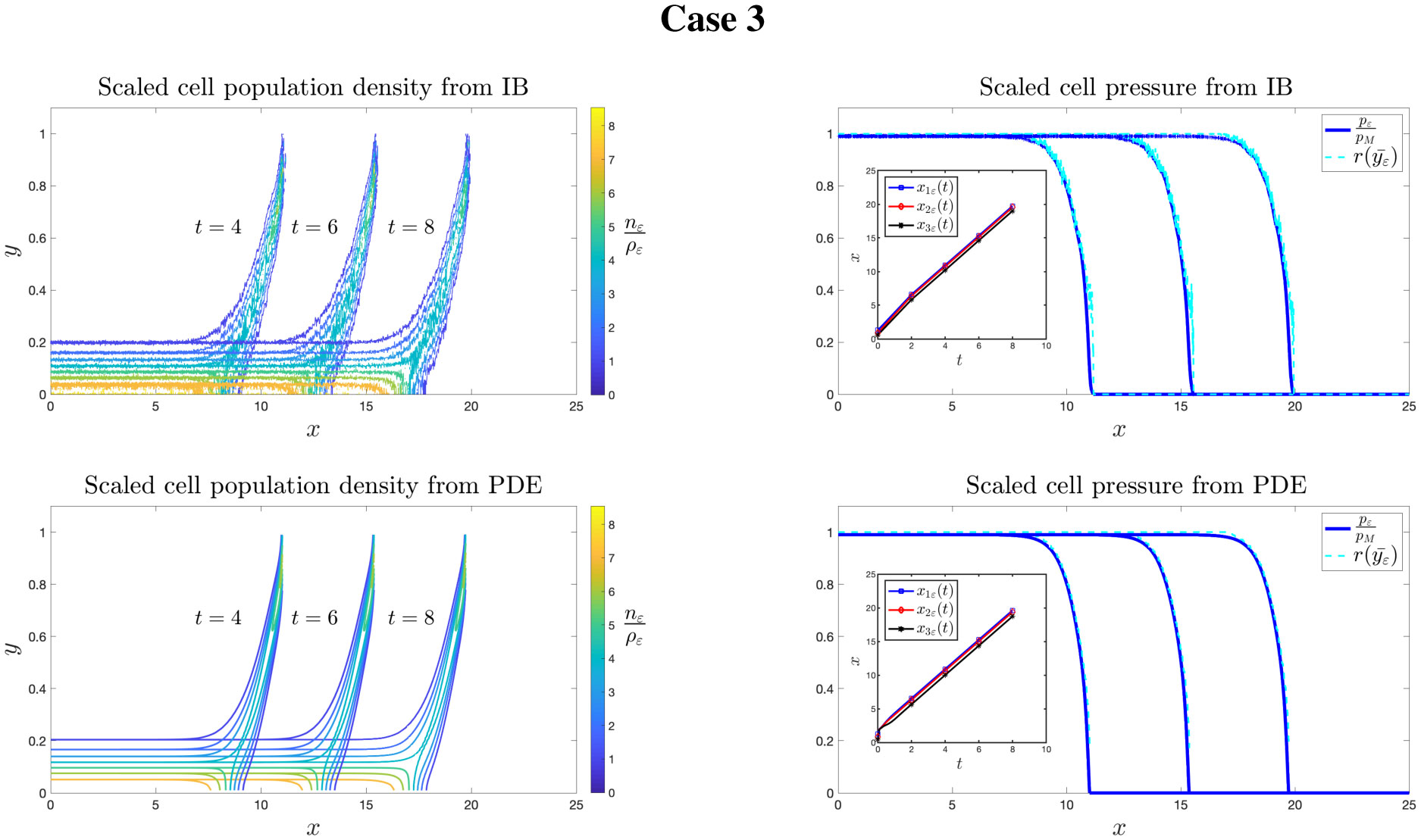
Existing comparative studies between individual-based models of growing cell populations and their continuum counterparts have mainly been focused on homogeneous populations, in which all cells have the same phenotypic characteristics. However, significant intercellular phenotypic variability is commonly observed in cellular systems. In light of these considerations, we develop here an individual-based model for the growth of phenotypically heterogeneous cell populations. In this model, the phenotypic state of each cell is described by a structuring variable that captures intercellular variability in cell proliferation and migration rates. The model tracks the spatial evolutionary dynamics of single cells, which undergo pressure-dependent proliferation, heritable phenotypic changes and directional movement in response to pressure differentials. We formally show that the continuum limit of this model comprises a non-local partial differential equation for the cell population density function, which generalises earlier models of growing cell populations. We report on the results of numerical simulations of the individual-based model which illustrate how proliferation-migration tradeoffs shaping the evolutionary dynamics of single cells can lead to the formation, at the population level, of travelling waves whereby highly-mobile cells locally dominate at the invasive front, while more-proliferative cells are found at the rear. Moreover, we demonstrate that there is an excellent quantitative agreement between these results and the results of numerical simulations and formal travelling-wave analysis of the continuum model, when sufficiently large cell numbers are considered. We also provide numerical evidence of scenarios in which the predictions of the two models may differ due to demographic stochasticity, which cannot be captured by the continuum model. This indicates the importance of integrating individual-based and continuum approaches when modelling the growth of phenotypically heterogeneous cell populations.

Keywords:

growing cell populations,
phenotypic heterogeneity,
individual-based models,
continuum models,
non-local partial differential equations,
travelling waves

Citation: Fiona R Macfarlane, Xinran Ruan, Tommaso Lorenzi. Individual-based and continuum models of phenotypically heterogeneous growing cell populations[J]. AIMS Bioengineering, 2022, 9(1): 68-92. doi: 10.3934/bioeng.2022007

Related Papers:

[1]	Annabelle Collin, Hadrien Bruhier, Jelena Kolosnjaj, Muriel Golzio, Marie-Pierre Rols, Clair Poignard . Spatial mechanistic modeling for prediction of 3D multicellular spheroids behavior upon exposure to high intensity pulsed electric fields. AIMS Bioengineering, 2022, 9(2): 102-122. doi: 10.3934/bioeng.2022009
[2]	Fırat Evirgen, Fatma Özköse, Mehmet Yavuz, Necati Özdemir . Real data-based optimal control strategies for assessing the impact of the Omicron variant on heart attacks. AIMS Bioengineering, 2023, 10(3): 218-239. doi: 10.3934/bioeng.2023015
[3]	Matthew Hogan, Glauco Souza, Ravi Birla . Assembly of a functional 3D primary cardiac construct using magnetic levitation. AIMS Bioengineering, 2016, 3(3): 277-288. doi: 10.3934/bioeng.2016.3.277
[4]	Daniel Pelaez, John H. Michel, Herman S. Cheung . Growth on elastic silicone substrate elicits a partial myogenic response in periodontal ligament derived stem cells. AIMS Bioengineering, 2016, 3(4): 515-527. doi: 10.3934/bioeng.2016.4.515
[5]	Atta Ullah, Hamzah Sakidin, Shehza Gul, Kamal Shah, Yaman Hamed, Maggie Aphane, Thabet Abdeljawad . Sensitivity analysis-based control strategies of a mathematical model for reducing marijuana smoking. AIMS Bioengineering, 2023, 10(4): 491-510. doi: 10.3934/bioeng.2023028
[6]	Adam B Fisher, Stephen S Fong . Lignin biodegradation and industrial implications. AIMS Bioengineering, 2014, 1(2): 92-112. doi: 10.3934/bioeng.2014.2.92
[7]	Chao Hu, Qing-Hua Qin . Bone remodeling and biological effects of mechanical stimulus. AIMS Bioengineering, 2020, 7(1): 12-28. doi: 10.3934/bioeng.2020002
[8]	Christina Großerhode, Daria Wehlage, Timo Grothe, Nils Grimmelsmann, Sandra Fuchs, Jessica Hartmann, Patrycja Mazur, Vanessa Reschke, Helena Siemens, Anke Rattenholl, Sarah Vanessa Homburg, Andrea Ehrmann . Investigation of microalgae growth on electrospun nanofiber mats. AIMS Bioengineering, 2017, 4(3): 376-385. doi: 10.3934/bioeng.2017.3.376
[9]	Takashi Nakazawa, Sohei Tasaki, Kiyohiko Nakai, Takashi Suzuki . Multicellular model of angiogenesis. AIMS Bioengineering, 2022, 9(1): 44-60. doi: 10.3934/bioeng.2022004
[10]	Edwige Arnold, Iness Hammami, Jingkui Chen, Sachin Gupte, Yves Durocher, Mario Jolicoeur . Overexpression of G6PDH does not affect the behavior of HEK-293 clones stably expressing interferon-α2b. AIMS Bioengineering, 2016, 3(3): 319-336. doi: 10.3934/bioeng.2016.3.319

Abstract

Existing comparative studies between individual-based models of growing cell populations and their continuum counterparts have mainly been focused on homogeneous populations, in which all cells have the same phenotypic characteristics. However, significant intercellular phenotypic variability is commonly observed in cellular systems. In light of these considerations, we develop here an individual-based model for the growth of phenotypically heterogeneous cell populations. In this model, the phenotypic state of each cell is described by a structuring variable that captures intercellular variability in cell proliferation and migration rates. The model tracks the spatial evolutionary dynamics of single cells, which undergo pressure-dependent proliferation, heritable phenotypic changes and directional movement in response to pressure differentials. We formally show that the continuum limit of this model comprises a non-local partial differential equation for the cell population density function, which generalises earlier models of growing cell populations. We report on the results of numerical simulations of the individual-based model which illustrate how proliferation-migration tradeoffs shaping the evolutionary dynamics of single cells can lead to the formation, at the population level, of travelling waves whereby highly-mobile cells locally dominate at the invasive front, while more-proliferative cells are found at the rear. Moreover, we demonstrate that there is an excellent quantitative agreement between these results and the results of numerical simulations and formal travelling-wave analysis of the continuum model, when sufficiently large cell numbers are considered. We also provide numerical evidence of scenarios in which the predictions of the two models may differ due to demographic stochasticity, which cannot be captured by the continuum model. This indicates the importance of integrating individual-based and continuum approaches when modelling the growth of phenotypically heterogeneous cell populations.

1. Introduction

Deterministic continuum models for the growth of cell populations have been increasingly used as theoretical tools to support empirical research regarding a broad spectrum of aspects of the development of solid tumours and living tissues. These models comprise partial differential equations (PDEs) that describe the evolution of cellular densities (or cell volume fractions) in response to pressure gradients that are generated by population growth, which can be mechanically-regulated [1], [2], nutrient-limited [3], pressure-dependent [4]–[6] or regulated by a combination of these mechanisms [7]–[11]. These models are amenable not only to numerical simulations but also to analytical approaches, which enable a complete exploration of the model parameter space. This permits a precise identification of the validity domain of the results obtained and ensures higher robustness and precision of the conclusions drawn therefrom, which ultimately provides a more in-depth theoretical understanding of the underlying cellular dynamics [12], [13].

Ideally, instead of defining such PDE models on the basis of population-scale phenomenological assumptions, one wants to derive them from first principles, that is, as the deterministic continuum limits of stochastic discrete models, i.e. individual-based (IB) models, which track the dynamics of single cells [14], [15]. This is to ensure that the terms comprised in the model equations provide a faithful mean-field representation of the underlying cellular dynamics. In fact, although being computationally intensive to simulate for large cell numbers and, to a wider extent, inaccessible to analytical techniques, IB models permit the representation of the finer details of cell-scale mechanisms and capture stochastic intercellular variability in the spatial and evolutionary trajectories of single cells. These aspects, which cannot be directly incorporated into phenomenological deterministic continuum models, become especially important in scenarios where cell numbers and densities are low (e.g. in the early stages of embryonic development and tissue regeneration, during the formation of distant metastases upon cancer cell extravasation, and when tumour size is severely reduced after therapy), due to the stronger impact that single-cell processes and demographic stochasticity are expected to have on the dynamics of cell populations. For this reason, a range of asymptotic techniques, probabilistic methods and limiting procedures have been developed and used in previous studies to systematically derive PDE models for the growth of cell populations from their individual-based counterparts [13]. For example, reaction-diffusion and nonlinear diffusion equations have been derived from their underlying random walks [16]–[21], from systems of discrete equations of motion [22]–[24], from discrete lattice-based exclusion processes [25]–[28] and from cellular automata [29]–[31]. However, these previous studies have mainly been focused on homogeneous populations in which all cells have the same phenotypic characteristics. Such homogeneity is rarely present in cellular systems, where significant intercellular phenotypic variability is commonly observed. In light of these considerations, we develop here an IB model for the growth of phenotypically heterogeneous cell populations. In this model, every cell is viewed as an individual agent whose phenotypic state is described by a structuring variable that captures intercellular variability in cell proliferation and migration rates. Cells undergo directional movement in response to pressure differentials [32]–[35], pressure-dependent proliferation [2], [36]–[38], and heritable phenotypic changes [39]–[41] according to a set of rules that correspond to a discrete-time branching random walk on the physical space and the space of phenotypic states [19], [42], [43]. We formally show that the deterministic continuum limit of this model is given by a non-local PDE for the cell population density function, which generalises earlier models [34], [38], [44] to the case of phenotypically heterogeneous cell populations. We then carry out numerical simulations of the IB model and compare the results obtained with the results of formal travelling-wave analysis and numerical simulations of the PDE model.

The paper is organised as follows. In Section 2, we introduce the IB model. In Section 3, we present its PDE counterpart (a formal derivation is provided in Section S1 of the Supplementary Material). In Section 4, in order to obtain results with broad structural stability under parameter changes, we first carry out formal travelling-wave analysis of the PDE model and then integrate the results obtained with numerical simulations of the IB model and numerical solutions of the PDE model. In Section 5, we summarise the main findings of our study and outline directions for future research.

2. The individual-based model

We model the dynamics of a phenotypically heterogeneous growing cell population. Cells within the population have the potential to undergo:
directional movement in response to pressure differentials – i.e. cells move down pressure gradients towards regions where they feel less compressed [32], [34], [37];
spontaneous, heritable phenotypic changes, which lead cells to randomly transition from one phenotypic state into another [39]–[41];
pressure-dependent proliferation – i.e. cells stop dividing, and can thus only die or remain quiescent, when the pressure that they experience overcomes a critical threshold, which is known as homeostatic pressure [34], [38], [45].

Focusing on a one-dimensional spatial domain scenario, the position of every cell at time t ∈ ℝ⁺ is described by the variable x ∈ ℝ. Moreover, the phenotypic state of each cell is characterised by a structuring variable y ∈ [0,Y] ⊂ ℝ⁺, with Y > 0, which takes into account intercellular variability in cell proliferation and migration rates. Here, the variable y could represent the level of expression of a gene that regulates both cell division and cell migration, such as those involved in the epithelial-to-mesenchymal transition promoting tumour invasion [46]–[48]. More specifically, the overexpression of some cancer-promoting genes has been shown to inhibit cell proliferation and promote cell migration in cancer cells, for example, FBXL10 expession in ovarian cancer cell lines [49] and EphB2 expression in glioblastomas [50]. Similarily, the downregulation of miR-451 observed in glioblastomas has been shown to reduce the proliferation rate and increase the migration potential of the cells [51].

Therefore in the model, without loss of generality, we consider the case where larger values of y correlate with a higher cell migration rate but a lower proliferation rate due to proliferation-migration tradeoffs [47], [48], [52]–[59].

We discretise the time, space and phenotype variables via

$t_{k} = k τ \in ℝ^{+}, x_{i} = i χ \in ℝ and y_{j} = j η \in [0, Y] with k, j \in ℕ_{0}, i \in ℤ, τ, χ, η \in ℝ_{*}^{+} .$

${x_{i}}_{i \in ℤ} \times {y_{j}}_{j \in ℕ_{0}}$

$N_{i, j}^{k} \in ℕ_{0}$

y_j

x_i

t_k

$n_{i, j}^{k} \equiv n (t_{k}, x_{i}, y_{j}) : = \frac{N_{i, j}^{k}}{χ η} and ρ_{i}^{k} \equiv ρ (t_{k}, x_{i}) : = η \sum_{j} n_{i, j}^{k} .$ (2.1)

i.e

$p_{i}^{k} \equiv p (t_{k}, x_{i}) = Π (ρ_{i}^{k}),$ (2.2)

[34]

[44]

[60]

$Π (0) = 0, \frac{d}{d ρ} Π (ρ) \geq 0 for ρ \in ℝ_{*}^{+} .$ (2.3)

As summarised by the schematics in Figure 1, between time-steps k and k + 1, each cell in phenotypic state y_j ∈ (0,Y) at position x_i ∈ ℝ can first move, next undergo phenotypic changes and then die or divide according to the rules described in the following subsections.

Figure 1. Schematics summarising the rules that govern the spatial evolutionary dynamics of single cells in the IB model. Between time-steps k and k + 1, each cell in phenotypic state y_j ∈ (0,Y) at position x_i ∈ ℝ may: a. move to either of the positions x_i−1 and x_i+1 with probabilities $𝒫_{L_{i, j}}^{k}$ and $𝒫_{R_{i, j}}^{k}$ defined via (2.12) and (2.13); b. undergo a phenotypic change and thus enter into either of the phenotypic states y_j−1 and y_j+1 with probabilities λ/2; c. die or divide with probabilities $𝒫_{D_{i, j}}^{k}$ and $𝒫_{B_{i, j}}^{k}$ defined via (2.4) and (2.5).

DownLoad: Full-Size Img PowerPoint

2.1. Mathematical modelling of cell death and division

To incorporate the effects of cell proliferation, we assume that a dividing cell is instantly replaced by two identical cells that inherit the phenotypic state of the parent cell (i.e. the progenies are placed on the same lattice site as their parent), while a dying cell is instantly removed from the population. We model pressure-dependent proliferation by letting the cells divide, die or remain quiescent with probabilities that depend on their phenotypic states and the pressure that they experience.

In particular, to define the probabilities of cell division and death, we introduce the function $R (y_{j}, p_{i}^{k})$ , which describes the net growth rate of the cell population density at position x_i at time t_k, and assume that between time-steps k and k + 1 a cell in phenotypic state y_j at position x_i may die with probability

$𝒫_{D_{i, j}}^{k} : = τ R {(y_{j}, p_{i}^{k})}_{-} where R {(y_{j}, p_{i}^{k})}_{-} = - m i n (0, R (y_{j}, p_{i}^{k})),$ (2.4)

$𝒫_{B_{i, j}}^{k} : = τ R {(y_{j}, p_{i}^{k})}_{+} where R {(y_{j}, p_{i}^{k})}_{+} = m a x (0, R (y_{j}, p_{i}^{k}))$ (2.5)

i.e

$𝒫_{Q_{i, j}}^{k} : = 1 - 𝒫_{B_{i, j}}^{k} - 𝒫_{D_{i, j}}^{k} .$ (2.6)

$0 < 𝒫_{B_{i, j}}^{k} + 𝒫_{D_{i, j}}^{k} < 1$

In order to capture the fact that, as mentioned earlier, larger values of y_j correlate with a lower cell proliferation rate, along with the fact that cells will stop dividing if the pressure at their current position becomes larger than the homeostatic pressure, which we model by means of the parameter p_M>0, we make the following assumptions

$R (Y,0) = 0, R (0, p_{M}) = 0, \partial_{p} R (y, p) < 0 and \partial_{y} R (y, p) < 0 for (y, p) \in (0, Y) \times ℝ^{+} .$ (2.7)

$R (y, p) : = r (y) - \frac{p}{p_{M}} with r (Y) = 0, r (0) = 1, \frac{d}{d y} r (y) < 0 for y \in (0, Y) .$ (2.8)

Remark 1.

Under assumptions

(2.7)

definitions

(2.5)

(2.6)

ensure that if $p_{i}^{k} \geq p_{M}$ then every cell at position x_i can only die or remain quiescent between time-steps k and k

Hence, in the remainder of the paper we will let the following condition hold

$\underset{i \in ℤ}{m a x} p_{i}^{0} \leq p_{M}$ (2.9)

so that

$p_{i}^{k} \leq p_{M} for all (k, i) \in ℕ_{0} \times ℤ .$ (2.10)

2.2. Mathematical modelling of phenotypic changes

We take into account heritable phenotypic changes by allowing cells to update their phenotypic states according to a random walk along the phenotypic dimension. More precisely, between time-steps k and k + 1, every cell either enters a new phenotypic state, with probability λ ∈ [0,1], or remains in its current phenotypic state, with probability 1-λ. Since, as mentioned earlier, we consider only spontaneous phenotypic changes that occur randomly due to non-genetic instability, we assume that a cell in phenotypic state y_j that undergoes a phenotypic change enters into either of the phenotypic states y_j±1 = y_j ± η with probabilities λ/2. No-flux boundary conditions are implemented by aborting any attempted phenotypic variation of a cell if it requires moving into a phenotypic state outside the interval [0,Y].

2.3. Mathematical modelling of cell movement

We model directional cell movement in response to pressure differentials as a biased random walk along the spatial dimension, whereby the movement probabilities depend on the difference between the pressure at the position occupied by a cell and the pressure at the neighbouring positions. As mentioned earlier, we consider the case where larger values of y_j correlate with a higher cell migration rate. Hence, we modulate the probabilities of cell movement by the function μ(y_j), which provides a measure of the mobility of cells in phenotypic state y_j and thus satisfies the following assumptions

$μ (0) > 0, \frac{d}{d y} μ (y) > 0 for y \in (0, Y] .$ (2.11)

y_j

x_i

_i−1

x_i

i.e

$𝒫_{L_{i, j}}^{k} = ν μ (y_{j}) \frac{{(p_{i}^{k} - p_{i - 1}^{k})}_{+}}{2 p_{M}} where {(p_{i}^{k} - p_{i - 1}^{k})}_{+} = m a x (0, p_{i}^{k} - p_{i - 1}^{k}),$ (2.12)

_i+1

x_i

i.e

$𝒫_{R_{i, j}}^{k} = ν μ (y_{j}) \frac{{(p_{i}^{k} - p_{i + 1}^{k})}_{+}}{2 p_{M}} where {(p_{i}^{k} - p_{i + 1}^{k})}_{+} = m a x (0, p_{i}^{k} - p_{i + 1}^{k})$ (2.13)

i.e

$𝒫_{S_{i, j}}^{k} = 1 - 𝒫_{L_{i, j}}^{k} - 𝒫_{R_{i, j}}^{k} .$ (2.14)

vμ

y_j

(2.9)

(2.10)

(2.12)

(2.13)

$0 < 𝒫_{L_{i, j}}^{k} + 𝒫_{R_{i, j}}^{k} < 1$

Remark 2. Definitions (2.12) and (2.13) ensure that cells will move down pressure gradients so as to reach regions where they feel less compressed.

3. The corresponding continuum model

Through a method analogous to those that we previously employed in [19], [61]–[64], letting the time-step τ → 0, the space-step χ → 0 and the phenotype-step η → 0 in such a way that

$\frac{ν χ^{2}}{2 τ} \to α \in ℝ_{*}^{+} and \frac{λ η^{2}}{2 τ} \to β \in ℝ_{*}^{+},$ (3.1)

Section S1 of the Supplementary Material

$(\begin{matrix} \partial_{t} n - α \hat{μ} (y) \partial_{x} (n \partial_{x} p) = R (y, p) n + β \partial_{y y}^{2} n, (x, y) \in ℝ \times (0, Y) \\ p = Π (ρ), ρ : = \int_{0}^{Y} n (t, x, y) d y, \end{matrix}$ (3.2)

$\hat{μ} (y) : = \frac{μ (y)}{p_{M}}$

(3.2)

i.e

(2.9)

$\underset{x \in ℝ}{m a x} p (0, x) \leq p_{M} .$ (3.3)

The mathematical model defined by complementing (3.2) with assumptions (2.3), (2.7) and (2.11) generalises earlier models of pressure-dependent cell population growth [34], [38], [44] to the case of phenotypically heterogeneous cell populations.

4. Main results

In this section, we first present the result of formal travelling-wave analysis of the PDE model (Subsection 4.1) and then integrate these results with numerical simulations of the IB model and numerical solutions of the PDE model (Subsection 4.2).

4.1. Formal travelling-wave analysis

We focus on a biological scenario in which cell movement occurs on a slower timescale compared to cell division and death, while spontaneous, heritable phenotypic changes occur on a slower timescale compared to cell movement [41], [65]. To this end, we introduce a small parameter ϵ > 0 and let

$α : = ϵ, β : = ϵ^{2} .$ (4.1)

i.e

$t \to \frac{t}{ϵ}$

(3.2)

$n_{ϵ} (t, x, y) = n (\frac{t}{ϵ}, x, y)$

$(\begin{matrix} ϵ \partial_{t} n_{ϵ} - ϵ \hat{μ} (y) \partial_{x} (n_{ϵ} \partial_{x} p_{ϵ}) = R (y, p_{ϵ}) n_{ϵ} + ϵ^{2} \partial_{y y}^{2} n_{ϵ}, (x, y) \in ℝ \times (0, Y) \\ p_{ϵ} = Π (ρ_{ϵ}), ρ_{ϵ} : = \int_{0}^{Y} n_{ϵ} (t, x, y) d y . \end{matrix}$ (4.2)

[66]

[67]

_(·)

Section S2 of the Supplementary Material

(2.3)

(2.8)

(2.11)

(4.2)

$n_{ϵ} (z, y) \approx ρ (z) δ_{\bar{y} (z)} (y), z = x - c t, c \in ℝ_{*}^{+},$ (4.3)

$- (c + \hat{μ} (y) p^{'}) \partial_{z} u = (r (y) - \frac{p}{p_{M}}) + {(\partial_{y} u)}^{2}, u \equiv u (z, y), (z, y) \in ℝ \times (0, Y)$

$p (z) = p_{M} r (\bar{y} (z)) z \in S u p p (p),$ (4.4)

$c \geq \underset{z \in S u p p (r (\bar{y}))}{s u p} 2 | \frac{d}{d y} r (\bar{y} (z)) | \sqrt{\frac{μ (\bar{y} (z))}{| \partial_{y y}^{2} u (z, \bar{y} (z)) |}} .$ (4.5)

$S u p p (p) = (- \infty, ℓ) with ℓ \in ℝ such that \bar{y} (ℓ) = Y$ (4.6)

$\lim_{z \to - \infty} \bar{y} (z) = 0, \lim_{z \to - \infty} p (z) = p_{M}, \bar{y}' (z) > 0 and p^{'} (z) < 0 z \in (- \infty, ℓ) .$ (4.7)

From a biological point of view, y(z) represents the dominant phenotype of cells at a certain position along the invading wave p(z). Since larger values of y correlate with a lower proliferation rate and a higher migration rate, the fact that y(z) increases monotonically from 0 to Y while p(z) decreases monotonically from p_M to 0 (cf. the results given by (4.6) and (4.7)) provides a mathematical formalisation of the idea that spatial sorting causes cells with a more mobile/less proliferative phenotype to become concentrated towards the front of the invading wave, which is thus a sparsely populated region, whereas phenotypic selection leads cells with a less mobile/more proliferative phenotype to dominate at the rear, which is then a densely populated region.

4.2. Numerical simulations

4.2.1. Set-up of numerical simulations

In order to carry out numerical simulations, we consider the time interval [0,T], with T = 8, we restrict the physical domain to the closed interval [0,X], with X = 25, and choose Y = 1. In order to facilitate the integration between numerical simulations and the results of formal travelling-wave analysis presented in Subsection 4.1, we solve numerically the rescaled PDE model (4.2), with ϵ = 0.01, and we carry out numerical simulations of the scaled IB model obtained by introducing the time scaling $t_{k} \to \frac{t_{k}}{ϵ} = k \frac{τ}{ϵ}$ and reformulating the governing rules of cell dynamics that are detailed in Section 2 in terms of

$p_{ϵ i}^{k} \equiv p_{ϵ} (t_{k}, x_{i}) = p (\frac{t_{k}}{ϵ}, x_{i}) = Π (ρ_{ϵ i}^{k}),$

$ρ_{ϵ i}^{k} \equiv ρ_{ϵ} (t_{k}, x_{i}) = ρ (\frac{t_{k}}{ϵ}, x_{i}) : = η \sum_{j} n_{ϵ i, j}^{k} and n_{ϵ i, j}^{k} \equiv n_{ϵ} (t_{k}, x_{i}, y_{j}) = n (\frac{t_{k}}{ϵ}, x_{i}, y_{j}) : = \frac{N_{ϵ i, j}^{k}}{χ η} .$

⁻⁵

$ν = \frac{2 τ}{χ^{2}} ϵ$

$λ = \frac{2 τ}{η^{2}} ϵ^{2}$

(3.1)

(4.1)

We consider a biological scenario in which, initially, the cell population is localised along the x = 0 boundary and most of the cells are in the phenotypic state y = y⁰ at every position. Specifically, we implement the following initial cell distribution for the IB model

$N_{ϵ i, j}^{0} = int (F_{ϵ} (x_{i}, y_{j})) with F_{ϵ} (x, y) = A_{0} C e^{- x^{2}} e^{- \frac{{(y - {\bar{y}}^{0})}^{2}}{ϵ}},$ (4.8)

$C \int_{0}^{Y} e^{- \frac{{(y - {\bar{y}}^{0})}^{2}}{ϵ}} d y = 1.$

₀

⁰

(2.1)

(2.2)

$n_{ϵ} (0, x, y) = n_{ϵ}^{0} (x, y)$

$n_{ϵ i, j}^{0} : = \frac{N_{ϵ i, j}^{0}}{χ η}$

$N_{ϵ i, j}^{0}$

(4.8)

$n_{ϵ}^{0} (x, y) : = {(\frac{F_{ϵ} (x, y)}{χ η} - \frac{1.5}{χ η})}_{+},$

F_ϵ

(4.8)

₊

We define R(y, p_ϵ) via (2.8) and, having chosen Y = 1, we further define

$r (y) : = 1 - y^{2} and μ (y) : = 0.01 + y^{2}$

(2.7)

(2.8)

(2.11)

(2.3)

$p_{ϵ} = Π (ρ_{ϵ}) : = (\begin{matrix} ρ_{ϵ} & (Case 1) \\ K_{γ} {(ρ_{ϵ})}^{γ} with K_{γ} > 0, γ > 1 & (Case 2) \\ κ {(ρ_{ϵ} - ρ^{*})}_{+} with κ, ρ^{*} > 0 & (Case 3) . \end{matrix}$ (4.9)

The definition given by Case 1 corresponds to the simplified scenario in which the cell pressure is a linear function of the cell density. In the definition given by Case 2, which was proposed in [44], the parameter K_γ is a scaling factor and the parameter γ provides a measure of the stiffness of the barotropic relation (i.e. the limit γ → ∞ corresponds to the scenario in which cells behave like an incompressible fluid). In the definition given by Case 3, which is such that the cell pressure is zero for ρ ≤ ρ* and is a monotonically increasing function of the cell density for ρ > ρ*, the parameter κ is a scaling factor and ρ* is the density below which the force that the cells exert upon one another is negligible [38], [60]. Unless otherwise specified: when the cell pressure is defined via Case 1 we choose p_M = 4.95 × 10⁴; when the cell pressure is defined via Case 2 we choose p_M = 3.675 × 10⁹, γ = 2 and $K_{γ} = \frac{3}{2}$ ; when the cell pressure is defined via Case 3 we choose p_M = 4.94 × 10⁵, κ = 10 and ρ* = 10².

Remark 3. The initial conditions and the values of p_M that are considered here are such that conditions (2.9) and (3.3) are satisfied.

4.2.2. Computational implementation of the IB model

All simulations are performed in Matlab. At each time-step, each cell undergoes a three-phase process: (i) cell movement, according to the probabilities defined via (2.12)–(2.14); (ii) phenotypic changes, with probabilities λ/2; (iii) division and death, according to the probabilities defined via (2.5) and (2.6). For each cell, during each phase, a random number is drawn from the standard uniform distribution on the interval (0,1) using the built-in Matlab function rand. It is then evaluated whether this number is lower than the probability of the event occurring and if so the event occurs. Since x_i ∈ [0,X], the attempted movement of a cell is aborted if it requires moving out of the spatial domain.

4.2.3. Methods used to solve numerically the non-local PDE (4.2)

Full details of the methods used to solve numerically the non-local PDE (4.2) posed on (0,T]×(0,X)×(0,Y) and subject to suitable initial and boundary conditions are given in Section S3 of the Supplementary Material.

4.2.4. Results of numerical simulations

Formation of complex spatial patterns of population growth. The plots in the top lines of Figures 2–4 summarise the results of numerical simulations of the IB model for the barotropic relations given by Cases 1–3 in (4.9). We plot in the left panels the scaled cell population density, n_ϵ/ρ_ϵ, and in the right panels (solid blue lines) the scaled cell pressure, p_ϵ/p_M, at progressive times.

The results of numerical simulations under all three cases display very similar dynamics, both with respect to the cell population density and the cell pressure, where we observe evolution to travelling-wave profiles of almost identical shapes and speeds (see also Remark 4). The incorporation of proliferation-migration tradeoffs lead cells to be non-uniformly distributed across both physical and phenotype space. More precisely, we observe a relatively small subpopulation of highly-mobile but minimally-proliferative cells (i.e. cells in phenotypic states y ≈ Y) that becomes concentrated towards the front of the invading wave, while rapidly-proliferating but minimally-mobile cells (i.e. cells in phenotypic states y ≈ 0) make up the bulk of the population in the rear. This is due to a dynamic interplay between spatial sorting and phenotypic selection. In fact, a more efficient response to pressure differentials by more-mobile cells leads to their positioning at the front of the wave, where the pressure is lower, before being overcome by the more-proliferative cells encroaching from the rear of the wave, which are ultimately selected due to their higher proliferative potential.

Quantitative agreement between the IB model and its PDE counterpart. The plots in the bottom lines of Figures 2–4 summarise the corresponding numerical solutions of the PDE model (4.2). Comparing these plots with those in the top lines, we can see that there is an excellent quantitative agreement between the results of numerical simulations of the IB model and the numerical solutions of its PDE counterpart, both with respect to the cell population density and the cell pressure, for each of the barotropic relations given by Cases 1–3 in (4.9).

All these plots indicate that, in agreement with the results presented in Subsection 4.1 (cf. the results given by (4.3)), when ϵ is sufficiently small, the scaled cell population density n_ϵ/ρ_ϵ is concentrated as a sharp Gaussian with maximum at a single point y_ϵ(t,x) for all x ∈ Supp(p_ϵ). The maximum point y_ϵ(t,x) corresponds to the dominant phenotype within the cell population at position x and time t. Again in agreement with the results presented in Subsection 4.1 (cf. the results given by (4.6) and (4.7)), the cell pressure p_ϵ behaves like a one-sided compactly supported and monotonically decreasing travelling front that connects p_M to 0, while the dominant phenotype y_ϵ increases monotonically from y = 0 to y = Y across the support of the invading wave. Moreover, we find an excellent quantitative agreement between p_ϵ(t,x)/p_M and r(y_ϵ(t,x)) (cf. the solid blue and dashed cyan lines in the right panels of Figures 2–4). This indicates that, when ϵ is sufficiently small, relation (4.4) is satisfied as well.

In order to measure the speed of these travelling waves, we track the dynamics of the points x_ϵ₁(t), x_ϵ₂(t) and x_ϵ₃(t) such that

$p_{ϵ} (t, x_{ϵ 1} (t)) = 0.2 p_{M}, p_{ϵ} (t, x_{ϵ 2} (t)) = 0.5 p_{M}, p_{ϵ} (t, x_{ϵ 3} (t)) = 0.8 p_{M} .$ (4.10)

x_ϵ

₁

x_ϵ

₂

x_ϵ

₃

Figures 2

${\tilde{x}}_{ϵ 1} (t)$

${\tilde{x}}_{ϵ 2} (t)$

${\tilde{x}}_{ϵ 3} (t)$

${\bar{y}}_{ϵ} (t, {\tilde{x}}_{ϵ 1} (t)) = 0.2$

${\bar{y}}_{ϵ} (t, {\tilde{x}}_{ϵ 2} (t)) = 0.5$

${\bar{y}}_{ϵ} (t, {\tilde{x}}_{ϵ 3} (t)) = 0.8$

${\bar{y}}_{ϵ} (t, x) : = a r g m a x_{y \in [0, Y]} n_{ϵ} (t, x, y),$ (4.11)

p_ϵ

(4.5)

_ϵ

$\partial_{y y}^{2} u_{ϵ} (8, x, {\bar{y}}_{ϵ} (8, x))$

u_ϵ

n_ϵ

$\partial_{y y}^{2} u (z, \bar{y} (z))$

Possible discrepancies between the IB model and its PDE counterpart. In the cases discussed so far, we have observed excellent quantitative agreement between averaged results of numerical simulations of the IB model and numerical solutions of the corresponding PDE model. However, we hypothesise that possible differences between the two models can emerge when cell dynamics are strongly impacted by demographic stochasticity, which cannot be captured by the PDE model.

In general, we expect demographic stochasticity to have a stronger impact on cell dynamics in the presence of smaller values of the homeostatic pressure p_M, since smaller values of p_M correlate with smaller cell numbers. Moreover, in the case where cells are initially distributed across both physical and phenotype space according to (4.8), we expect demographic stochasticity to escalate during the early stages of cell dynamics if sufficiently small values of the parameter A₀ and sufficiently large values of the parameter y⁰ (i.e. values of y⁰ sufficiently far from 0 and sufficiently close to Y) are considered. In fact, smaller values of A₀ correlate with lower initial cell numbers. Moreover, since cells in phenotypic states y ≈ 0 will ultimately be selected in the rear of the invading wave (cf. the plots in the left panels of Figures 2–4), bottleneck effects leading to a temporary drastic reduction in the size of the cell population may occur if y⁰ is sufficiently far from 0.

Remark 4. The robustness of the results of numerical simulations of the IB model presented so far is supported by the fact that there is an excellent quantitative agreement between them and the results of numerical simulations and formal travelling-wave analysis of the corresponding PDE model. In fact, in the light of this agreement, independently of the specific definitions of the model functions Π, R and μ, provided that assumptions (2.3), (2.7) and (2.11) are satisfied, and sufficiently large cell numbers are considered, in the asymptotic regime ϵ → 0, one can expect the rules governing the spatial evolutionary dynamics of single cells considered here to bring about patterns of population growth that will ultimately be qualitatively similar to those of Figures 2–4.

Hence, to test the aforementioned hypothesis, we carry out numerical simulations of the two models for decreasing values of A₀ and increasing values of y⁰ in the initial cell distribution (4.8). Furthermore, we define the cell pressure through the barotropic relation given by Case 1 in (4.9) and set $p_{M} : = \max_{x \in [0, X]} Π (ρ_{ϵ} (0, x))$ , so that smaller values of A₀ correspond to smaller value of p_M as well.

Figure 2. Numerical simulation results of the IB model (top row) and the PDE model (4.2) (bottom row) in the case where the cell pressure is defined through the barotropic relation given by Case 1 in (4.9). Plots display the scaled cell population density n_ϵ/ρ_ϵ (left panels) and the scaled cell pressure p_ϵ/p_M (right panels, solid blue lines) at three successive time instants (i.e. t = 4, t = 6 and t = 8) for both modelling approaches. The dashed cyan lines in the right panels highlight the corresponding values of r(y_ϵ), with y_ϵ defined via (4.11). The insets of the right panels display the plots of x_ϵ₁(t) (blue squares), x_ϵ₂(t) (red diamonds) and x_ϵ₃(t) (black stars) defined via (4.10). The results from the IB model were obtained by averaging over 10 simulations.

DownLoad: Full-Size Img PowerPoint

Figure 3. Numerical simulation results of the IB model (top row) and the PDE model (4.2) (bottom row) in the case where the cell pressure is defined through the barotropic relation given by Case 2 in (4.9). Plots display the scaled cell population density n_ϵ/ρ_ϵ (left panels) and the scaled cell pressure p_ϵ/p_M (right panels, solid blue lines) at three successive time instants (i.e. t = 4, t = 6 and t = 8) for both modelling approaches. The dashed cyan lines in the right panels highlight the corresponding values of r(y_ϵ), with y_ϵ defined via (4.11). The insets of the right-hand panels display the plots of x_ϵ₁(t) (blue squares), x_ϵ₂(t) (red diamonds) and x_ϵ₃(t) (black stars) defined via (4.10). The results from the IB model were obtained by averaging over 10 simulations.

DownLoad: Full-Size Img PowerPoint

Figure 4. Numerical simulation results of the IB model (top row) and the PDE model (4.2) (bottom row) in the case where the cell pressure is defined through the barotropic relation given by Case 3 in (4.9). Plots display the scaled cell population density n_ϵ/ρ_ϵ (left panels) and the scaled cell pressure p_ϵ/p_M (right panels, solid blue lines) at three successive time instants (i.e. t = 4, t = 6 and t = 8) for both modelling approaches. The dashed cyan lines in the right panels highlight the corresponding values of r(y_ϵ), with y_ϵ defined via (4.11). The insets of the right-hand panels display the plots of x_ϵ₁(t) (blue squares), x_ϵ₂(t) (red diamonds) and x_ϵ₃(t) (black stars) defined via (4.10). The results from the IB model were obtained by averaging over 10 simulations.

DownLoad: Full-Size Img PowerPoint

The results obtained for the IB model are summarised by the plots in Figure 5, which display typical dynamics of the scaled cell pressure p_ϵ/p_M, while the corresponding results for the PDE model (4.2) are summarised by the plots in Figure 6. These results corroborate our hypothesis by demonstrating that the quantitative agreement between the IB model and its PDE counterpart deteriorates when smaller values of A₀ and larger values of y⁰ are considered (cf. the plots in the bottom-line panels of Figures 5 and 6).

Figure 5. Numerical simulation results of the IB model for different values of the parameters A₀ and y⁰ in the initial cell distribution (4.8) – i.e. y⁰ = 0.2 (left column) or y⁰ = 0.8 (right column) and A₀ = 10 (top row) or A₀ = 1 (central row) or A₀ = 0.27 (bottom row). The solid blue lines highlight the values of the scaled cell pressure p_ϵ/p_M at three successive time instants (i.e. t = 3, t = 5 and t = 7). The dashed cyan lines highlight the corresponding values of r(y_ϵ), with y_ϵ defined via (4.11). These results were obtained by averaging over 10 simulations.

DownLoad: Full-Size Img PowerPoint

Figure 6. Numerical simulation results of the PDE model (4.2) for different values of the parameters A₀ and y⁰ in the initial cell distribution (4.8) – i.e. y⁰ = 0.2 (left column) or y⁰ = 0.8 (right column) and A₀ = 10 (top row) or A₀ = 1 (central row) or A₀ = 0.27 (bottom row). The solid blue lines highlight the values of the scaled cell pressure p_ϵ/p_M at three successive time instants (i.e. t = 3, t = 5 and t = 7). The dashed cyan lines highlight the corresponding values of r(y_ϵ), with y_ϵ defined via (4.11).

DownLoad: Full-Size Img PowerPoint

In line with our expectations, this is due to the fact that stronger stochastic effects associated with small population levels in the initial phase of cell dynamics create the potential for population extinction to occur in some simulations of the IB model – i.e. under the exact same parameter setting, we can observe extinction or survival of the population in the IB model due to demographic stochasticity (cf. the single simulation results displayed in Figures 7 and 8). On the other hand, the cell population will always persist according to the PDE model. This ultimately results in discrepancies between the average behaviour of the IB model and the behaviour of the PDE model (cf. the plots in the bottom-line panels of Figures 5 and 6).

Figure 7. Numerical results of a single simulation of the IB model with A₀ = 0.27 and y⁰ = 0.8 in the initial cell distribution (4.8) – i.e. 1 out of the 10 simulations that are used to produce the average results displayed in the right-column, bottom-line panel of Figure 5. Plots display the scaled cell population density n_ϵ/ρ_ϵ (top panels) and the scaled cell pressure p_ϵ/p_M (bottom panels, solid blue lines) at five successive time instants (i.e. t = 0, t = 1, t = 2, t = 3 and t = 4). The dashed cyan lines in the bottom panels highlight the corresponding values of r(y_ϵ), with y_ϵ defined via (4.11). In this simulation, the cell population does not go extinct.

DownLoad: Full-Size Img PowerPoint

Figure 8. Numerical results of a single simulation of the IB model with A₀ = 0.27 and y⁰ = 0.8 in the initial cell distribution (4.8) – i.e. 1 out of the 10 simulations that are used to produce the average results displayed in the right-column, bottom-line panel of Figure 5. Plots display the scaled cell population density n_ϵ/ρ_ϵ (top panels) and the scaled cell pressure p_ϵ/p_M (bottom panels, solid blue lines) at five successive time instants (i.e. t = 0, t = 1, t = 2, t = 3 and t = 4). The dashed cyan lines in the bottom panels highlight the corresponding values of r(y_ϵ), with y_ϵ defined via (4.11). In this simulation, the cell population goes extinct rapidly.

DownLoad: Full-Size Img PowerPoint

5. Conclusions and research perspectives

We developed an IB model for the dynamics of phenotypically heterogeneous growing cell populations, which captures intercellular variability in cell proliferation and migration rates. We concentrated on a proliferation-migration tradeoff scenario, where the cell phenotypes span a spectrum of states from minimally-mobile but highly-proliferative to highly-mobile but minimally-proliferative. In the context of cancer invasion, such a tradeoff is the tenet of the “go-or-grow” hypothesis, which was conceived following observations of glioma cell behaviour [56] and has stimulated much empirical and theoretical research – see, for instance, [53], [56], [57], [59], [68]–[72] and references therein.

We reported on the results of numerical simulations of the IB model which illustrate how proliferation-migration tradeoffs shaping the evolutionary dynamics of single cells can lead, at the population level, to the generation of travelling waves whereby phenotypes are structured across the support of the wave, with highly-mobile cells being found at the invasive front and more-proliferative cells dominating at the rear. Similar patterns of cell population growth have been observed in gliomas, where cells within the interior of the tumour exhibit higher proliferation and lower migration rates, while cells on the tumour border are instead characterised by lower proliferation and higher migration rates [48], [50], [56], [73], [74].

We formally derived the deterministic continuum counterpart of the IB model, which comprises a non-local PDE for the cell population density function, and carried out a comparative study between numerical simulations of the IB model and both numerical solutions and formal travelling-wave analysis of the PDE model. We demonstrated that there is an excellent quantitative agreement between the results of numerical simulations of the IB model and the results of numerical simulations and travelling-wave analysis of the corresponding PDE model, when sufficiently large cell numbers are considered. This testifies to the robustness of the results of numerical simulations of the IB model presented here (see Remark 4).

In general, agreement between IB models and their continuum counterparts arises in regions of the model parameter space that correspond to sufficiently large cell numbers [75]–[77], while discrepancies may arise when the number of cells becomes low – e.g. if the rate of cell death is sufficiently large [78] – leading to possible extinction of the population in the IB model. We have provided numerical evidence of situations such as these in which the predictions of the two models can differ due to demographic stochasticity, which cannot be captured by the PDE model. This indicates the importance of integrating individual-based and continuum approaches when modelling the growth of phenotypically heterogeneous cell populations.

Although in this work we focused on a one-dimensional spatial domain scenario, the IB model presented here, and the formal limiting procedure to derive the corresponding continuum model, could easily be adapted to higher spatial dimensions. Furthermore, while we represented the spatial domain of the IB model as a regular lattice, it would certainly be interesting to generalise the underlying modelling approach, as well as the formal method to derive the continuum counterpart of the model, to cases where cells are distributed over irregular lattices and also to cases where off-latice representations of the spatial domain are adopted. The present IB model could also be extended further to include the effects of chemical species (e.g. nutrients, growth factors, chemoattractants, chemorepulsants) and how the cells interact with and respond to these chemicals. To include and implement chemical species in the current model, we could use a hybrid modelling approach whereby the probabilistic rules governing the dynamics of single cells would be coupled with balance equations for the chemical concentrations. Hybrid modelling approaches of this type have been utilised in the context of modelling various aspects of cancer growth and development – see, for instance, [11], [62], [79]–[82].

The generality of our assumptions makes the IB modelling framework presented here applicable to a broad range of biological processes that are driven by the growth of phenotypically heterogeneous cell populations, including tumour invasion and tissue remodelling and repair. It would thus be interesting to focus on particular cellular systems, and consequently define specific models, which could then be more accurately parameterised using precise biological data. This would offer the opportunity to dissect out the role played by different spatiotemporal evolutionary processes at the single-cell level in the formation of complex spatial patterns of population growth.

Acknowledgments

T.L. gratefully acknowledges support from the MIUR grant “Dipartimenti di Eccellenza 2018-2022” (Project no. E11G18000350001). F.R.M. gratefully acknowledges support from the RSE Saltire Early Career Fellowship ‘Multiscale mathematical modelling of spatial eco-evolutionary cancer dynamics’ (Fellowship No. 1879).

Conflict of interest

The authors declare no competing interests.

References

[1]	Chaplain MAJ, Giverso C, Lorenzi T, et al. (2019) Derivation and application of effective interface conditions for continuum mechanical models of cell invasion through thin membranes. SIAM J Appl Math 79: 2011-2031. https://doi.org/10.1137/19M124263X
[2]	Ranft J, Basan M, Elgeti J, et al. (2010) Fluidization of tissues by cell division and apoptosis. Proc Nat Acad Sci USA 107: 20863-20868. https://doi.org/10.1073/pnas.1011086107
[3]	Giverso C, Ciarletta P (2016) On the morphological stability of multicellular tumour spheroids growing in porous media. Eur Phys J E 39: 92. https://doi.org/10.1140/epje/i2016-16092-7
[4]	Bubba F, Perthame B, Pouchol C (2020) Hele–shaw limit for a system of two reaction-(cross-) diffusion equations for living tissues equations for living tissues. Arch Ration Mech Anal 236: 735-766. https://doi.org/10.1007/s00205-019-01479-1
[5]	David N, Ruan X (2022) An asymptotic preserving scheme for a tumor growth model of porous medium type. ESAIM Math Model Numer Anal 56: 121-150. https://doi.org/10.1051/m2an/2021080
[6]	Lorenzi T, Lorz A, Perthame B (2017) On interfaces between cell populations with different mobilities. Kinet Relat Mod 10: 299-311. https://doi.org/10.3934/krm.2017012
[7]	Bresch D, Colin T, Grenier E, et al. (2010) Computational modeling of solid tumor growth: the avascular stage. SIAM J Sci Comput 32: 2321-2344. https://doi.org/10.1137/070708895
[8]	Ciarletta P, Foret L, Ben Amar M (2011) The radial growth phase of malignant melanoma: multi-phase modelling, numerical simulations and linear stability analysis. J R Soc Interface 8: 345-368. https://doi.org/10.1098/rsif.2010.0285
[9]	Gallinato O, Colin T, Saut O, et al. (2017) Tumor growth model of ductal carcinoma: from in situ phase to stroma invasion. J Theor Biol 429: 253-266. https://doi.org/10.1016/j.jtbi.2017.06.022
[10]	Perthame B (2014) Some mathematical aspects of tumor growth and therapy. ICM 2014-International Congress of Mathematicians.
[11]	Lowengrub JS, Frieboes HB, Jin F, et al. (2009) Nonlinear modelling of cancer: bridging the gap between cells and tumours. Nonlinearity 23: R1. https://doi.org/10.1088/0951-7715/23/1/R01
[12]	Kuznetsov M, Clairambault J, Volpert V (2021) Improving cancer treatments via dynamical biophysical models. Phys Life Rev 39: 1-48. https://doi.org/10.1016/j.plrev.2021.10.001
[13]	Lorenzi T (2022) Cancer modelling as fertile ground for new mathematical challenges. Phys Life Rev 40: 3-5. https://doi.org/10.1016/j.plrev.2022.01.003
[14]	Anderson ARA (2007) A hybrid multiscale model of solid tumour growth and invasion: evolution and the microenvironment. Single-cell-based models in biology and medicine. Switzerland: Birkhäuser Basel 3-28.
[15]	Van Liedekerke P, Palm MM, Jagiella N, et al. (2015) Simulating tissue mechanics with agent-based models: concepts, perspectives and some novel results. Comput Part Mech 2: 401-444. https://doi.org/10.1007/s40571-015-0082-3
[16]	Inoue M (1991) Derivation of a porous medium equation from many Markovian particles and the propagation of chaos. Hiroshima Math J 21: 85-110. https://doi.org/10.32917/hmj/1206128924
[17]	Oelschläger K (1989) On the derivation of reaction-diffusion equations as limit dynamics of systems of moderately interacting stochastic processes. Probab Theory Relat Fields 82: 565-586. https://doi.org/10.1007/BF00341284
[18]	Penington CJ, Hughes BD, Landman KA (2011) Building macroscale models from microscale probabilistic models: a general probabilistic approach for nonlinear diffusion and multispecies phenomena. Phys Rev E 84: 041120. https://doi.org/10.1103/PhysRevE.84.041120
[19]	Chaplain MAJ, Lorenzi T, Macfarlane FR (2020) Bridging the gap between individual-based and continuum models of growing cell populations. J Math Biol 80: 343-371. https://doi.org/10.1007/s00285-019-01391-y
[20]	Lorenzi T, Murray PJ, Ptashnyk M (2020) From individual-based mechanical models of multicellular systems to free-boundary problems. Interface Free Bound 22: 205-244. https://doi.org/10.4171/IFB/439
[21]	Baker RE, Parker A, Simpson MJ (2019) A free boundary model of epithelial dynamics. J Theor Biol 481: 61-74. https://doi.org/10.1016/j.jtbi.2018.12.025
[22]	Oelschläger K (1990) Large systems of interacting particles and the porous medium equation. J Differ Equ 88: 294-346. https://doi.org/10.1016/0022-0396(90)90101-T
[23]	Murray PJ, Edwards CM, Tindall MJ, et al. (2009) From a discrete to a continuum model of cell dynamics in one dimension. Phys Rev E 80: 031912. https://doi.org/10.1103/PhysRevE.80.031912
[24]	Murray PJ, Edwards CM, Tindall MJ, et al. (2012) Classifying general nonlinear force laws in cell-based models via the continuum limit. Phys Rev E 85: 021921. https://doi.org/10.1103/PhysRevE.85.021921
[25]	Dyson L, Maini PK, Baker RE (2012) Macroscopic limits of individual-based models for motile cell populations with volume exclusion. Phys Rev E 86: 031903. https://doi.org/10.1103/PhysRevE.86.031903
[26]	Johnston ST, Baker RE, McElwain DL, et al. (2017) Co-operation, competition and crowding: a discrete framework linking Allee kinetics, nonlinear diffusion, shocks and sharp-fronted travelling waves. Sci Rep 7: 1-19. https://doi.org/10.1038/srep42134
[27]	Johnston ST, Simpson MJ, Baker RE (2012) Mean-field descriptions of collective migration with strong adhesion. Phys Rev E 85: 051922. https://doi.org/10.1103/PhysRevE.85.051922
[28]	Johnston ST, Simpson MJ, Baker RE (2015) Modelling the movement of interacting cell populations: a moment dynamics approach. J Theor Biol 370: 81-92. https://doi.org/10.1016/j.jtbi.2015.01.025
[29]	Deroulers C, Aubert M, Badoual M, et al. (2009) Modeling tumor cell migration: from microscopic to macroscopic models. Phys Rev E 79: 031917. https://doi.org/10.1103/PhysRevE.79.031917
[30]	Drasdo D (2005) Coarse graining in simulated cell populations. Adv Complex Syst 8: 319-363. https://doi.org/10.1142/S0219525905000440
[31]	Simpson MJ, Merrifield A, Landman KA, et al. (2007) Simulating invasion with cellular automata: Connecting cell-scale and population-scale properties. Phys Rev E 76: 021918. https://doi.org/10.1103/PhysRevE.76.021918
[32]	Ambrosi D, Preziosi L (2002) On the closure of mass balance models for tumor growth. Math Mod Meth Appl Sci 12: 737-754. https://doi.org/10.1142/S0218202502001878
[33]	Byrne HM, Chaplain MAJ (1997) Free boundary value problems associated with the growth and development of multicellular spheroids. Eur J Appl Math 8: 639-658. https://doi.org/10.1017/S0956792597003264
[34]	Byrne HM, Drasdo D (2009) Individual-based and continuum models of growing cell populations: a comparison. J Math Biol 58: 657. https://doi.org/10.1007/s00285-008-0212-0
[35]	Greenspan HP (1976) On the growth and stability of cell cultures and solid tumors. J Theor Biol 56: 229-242. https://doi.org/10.1016/S0022-5193(76)80054-9
[36]	Bru A, Albertos S, Subiza JL, et al. (2003) The universal dynamics of tumor growth. Biophys J 85: 2948-2961. https://doi.org/10.1016/S0006-3495(03)74715-8
[37]	Byrne HM, Preziosi L (2003) Modelling solid tumour growth using the theory of mixtures. Math Med Biol 20: 341-366. https://doi.org/10.1093/imammb/20.4.341
[38]	Drasdo D, Hoehme S (2012) Modeling the impact of granular embedding media, and pulling versus pushing cells on growing cell clones. New J Phys 14: 055025. https://doi.org/10.1088/1367-2630/14/5/055025
[39]	Brock A, Chang H, Huang S (2009) Non-genetic heterogeneity—A mutation-independent driving force for the somatic evolution of tumours. Nat Rev Genet 10: 336-342. https://doi.org/10.1038/nrg2556
[40]	Chisholm RH, Lorenzi T, Clairambault J (2016) Cell population heterogeneity and evolution towards drug resistance in cancer: biological and mathematical assessment, theoretical treatment optimisation. Biochim Biophys Acta Gen Subj 1860: N2627-2645. https://doi.org/10.1016/j.bbagen.2016.06.009
[41]	Huang S (2013) Genetic and non-genetic instability in tumor progression: Link between the fitness landscape and the epigenetic landscape of cancer cells. Cancer Metastasis Rev 32: 423-448. https://doi.org/10.1007/s10555-013-9435-7
[42]	Chisholm RH, Lorenzi T, Desvillettes L (2016) Evolutionary dynamics of phenotype-structured populations: From individual-level mechanisms to population-level consequences. Z Angew Math Phys 67: 1-34. https://doi.org/10.1007/s00033-016-0690-7
[43]	Hughes BD (1995) Random walks and random environments: random walks. UK: Oxford University Press.
[44]	Perthame B, Quiros F, Vazquez JL (2014) The Hele–Shaw asymptotics for mechanical models of tumor growth. Arch Ration Mech Anal 212: 93-127. https://doi.org/10.1007/s00205-013-0704-y
[45]	Basan M, Risler T, Joanny JF, et al. (2009) Homeostatic competition drives tumor growth and metastasis nucleation. HFSP J 3: 265-272. https://doi.org/10.2976/1.3086732
[46]	Novikov NM, Zolotaryova SY, Gautreau AM (2021) Mutational drivers of cancer cell migration and invasion. Br J Cancer 124: 102-114. https://doi.org/10.1038/s41416-020-01149-0
[47]	Alfonso JCL, Talkenberger K, Seifert M, et al. (2017) The biology and mathematical modelling of glioma invasion: a review. J R Soc Interface 14: 20170490. https://doi.org/10.1098/rsif.2017.0490
[48]	Giese A, Bjerkvig R, Berens ME, et al. (2003) Cost of migration: invasion of malignant gliomas and implications for treatment. J Clin Oncol 21: 1624-1636. https://doi.org/10.1200/JCO.2003.05.063
[49]	Yan M, Yang X, Shen R, et al. (2018) miR-146b promotes cell proliferation and increases chemosensitivity, but attenuates cell migration and invasion via FBXL10 in ovarian cancer. Cell Death Dis 9: 1-17. https://doi.org/10.1038/s41419-018-1093-9
[50]	Wang SD, Rath P, Lal B, et al. (2012) EphB2 receptor controls proliferation/migration dichotomy of glioblastoma by interacting with focal adhesion kinase. Oncogene 31: 5132-5143. https://doi.org/10.1038/onc.2012.16
[51]	Godlewski J, Bronisz A, Nowicki MO, et al. (2010) microRNA-451: A conditional switch controlling glioma cell proliferation and migration. Cell Cycle 9: 2814-2820. https://doi.org/10.4161/cc.9.14.12248
[52]	Aktipis CA, Boddy AM, Gatenby RA, et al. (2013) Life history trade-offs in cancer evolution. Nat Rev Cancer 13: 883. https://doi.org/10.1038/nrc3606
[53]	Gallaher JA, Brown JS, Anderson ARA (2019) The impact of proliferation-migration tradeoffs on phenotypic evolution in cancer. Sci Rep 9: 1-10. https://doi.org/10.1038/s41598-019-39636-x
[54]	Gerlee P, Anderson ARA (2009) Evolution of cell motility in an individual-based model of tumour growth. J Theor Biol 259: 67-83. https://doi.org/10.1016/j.jtbi.2009.03.005
[55]	Gerlee Pand Nelander S.The impact of phenotypic switching on glioblastoma growth and invasion. PLoS Comput Biol (2012) 8: e1002556. https://doi.org/10.1371/journal.pcbi.1002556
[56]	Giese A, Loo MA, Tran N, et al. (1996) Dichotomy of astrocytoma migration and proliferation. Int J Cancer 67: 275-282.
[57]	Hatzikirou H, Basanta D, Simon M, et al. (2012) ‘Go or Grow’: the key to the emergence of invasion in tumour progression?. Math Med Biol 29: 49-65. https://doi.org/10.1093/imammb/dqq011
[58]	Orlando PA, Gatenby RA, Brown JS (2013) Tumor evolution in space: The effects of competition colonization tradeoffs on tumor invasion dynamics. Front Oncol 3: 45. https://doi.org/10.3389/fonc.2013.00045
[59]	Pham K, Chauviere A, Hatzikirou H, et al. (2012) Density-dependent quiescence in glioma invasion: Instability in a simple reaction–diffusion model for the migration/proliferation dichotomy. J Biol Dyn 6: 54-71. https://doi.org/10.1080/17513758.2011.590610
[60]	Tang M, Vauchelet N, Cheddadi I, et al. (2013) Composite waves for a cell population system modeling tumor growth and invasion. Chinese Ann Math Ser B 34: 295-318. https://doi.org/10.1007/s11401-013-0761-4
[61]	Ardaseva A, Anderson ARA, Gatenby RA, et al. (2020) Comparative study between discrete and continuum models for the evolution of competing phenotype-structured cell populations in dynamical environments. Phys Rev E 102: 042404. https://doi.org/10.1103/PhysRevE.102.042404
[62]	Bubba F, Lorenzi T, Macfarlane FR (2020) From a discrete model of chemotaxis with volume-filling to a generalized Patlak–Keller–Segel model. Proc R Soc A 476: 20190871. https://doi.org/10.1098/rspa.2019.0871
[63]	Macfarlane FR, Chaplain MAJ, Lorenzi T (2020) A hybrid discrete-continuum approach to model Turing pattern formation. Math Biosci Eng 17: 7442-7479. https://doi.org/10.3934/mbe.2020381
[64]	Stace REA, Stiehl T, Chaplain MAJ, et al. (2020) Discrete and continuum phenotype-structured models for the evolution of cancer cell populations under chemotherapy. Math Mod Nat Phen 15: 14. https://doi.org/10.1051/mmnp/2019027
[65]	Smith JT, Tomfohr JK, Wells MC, et al. (2004) Measurement of cell migration on surface-bound fibronectin gradients. Langmuir 20: 8279-8286. https://doi.org/10.1021/la0489763
[66]	Lorenzi T, Perthame B, Ruan X (2021) Invasion fronts and adaptive dynamics in a model for the growth of cell populations with heterogeneous mobility. Eur J Appl Math 2021: 1-18. https://doi.org/10.1017/S0956792521000218
[67]	Lorenzi T, Painter KJ (2022) Trade-offs between chemotaxis and proliferation shape the phenotypic structuring of invading waves. Int J Non Linear Mech 139: 103885. https://doi.org/10.1016/j.ijnonlinmec.2021.103885
[68]	Corcoran A, Del Maestro RF (2003) Testing the “go or grow” hypothesis in human medulloblastoma cell lines in two and three dimensions. Neurosurgery 53: 174-185. https://doi.org/10.1227/01.NEU.0000072442.26349.14
[69]	Hoek KS, Eichhoff OM, Schlegel NC, et al. (2008) In vivo switching of human melanoma cells between proliferative and invasive states. Cancer Res 68: 650-656. https://doi.org/10.1158/0008-5472.CAN-07-2491
[70]	Stepien TL, Rutter EM, Kuang Y (2018) Traveling waves of a go-or-grow model of glioma growth. SIAM J Appl Math 78: 1778-1801. https://doi.org/10.1137/17M1146257
[71]	Vittadello ST, McCue SW, Gunasingh G, et al. (2020) Examining go-or-grow using fluorescent cell-cycle indicators and cell-cycle-inhibiting drugs. Biophys J 118: 1243-1247. https://doi.org/10.1016/j.bpj.2020.01.036
[72]	Zhigun A, Surulescu C, Hunt A (2018) A strongly degenerate diffusion-haptotaxis model of tumour invasion under the go-or-grow dichotomy hypothesis. Math Methods Appl Sci 41: 2403-2428. https://doi.org/10.1002/mma.4749
[73]	Dhruv HD, McDonough Winslow WS, Armstrong B, et al. (2013) Reciprocal activation of transcription factors underlies the dichotomy between proliferation and invasion of glioma cells. PLoS One 8: e72134. https://doi.org/10.1371/journal.pone.0072134
[74]	Xie Q, Mittal S, Berens ME (2014) Targeting adaptive glioblastoma: an overview of proliferation and invasion. Neuro-Oncol 16: 1575-1584. https://doi.org/10.1093/neuonc/nou147
[75]	Simpson MJ, Baker RE, Buenzli PR, et al. (2022) Reliable and efficient parameter estimation using approximate continuum limit descriptions of stochastic models.. https://doi.org/10.1101/2022.02.02.478913
[76]	Nardini JT, Baker RE, Simpson MJ, et al. (2021) Learning differential equation models from stochastic agent-based model simulations. J Roy Soc Interface 18: 20200987. https://doi.org/10.1098/rsif.2020.0987
[77]	Simpson MJ, Sharp JA, Baker RE (2014) Distinguishing between mean-field, moment dynamics and stochastic descriptions of birth–death–movement processes. Phys A Stat Mech Appl 395: 236-246. https://doi.org/10.1016/j.physa.2013.10.026
[78]	Johnston ST, Simpson MJ, Crampin EJ (2020) Predicting population extinction in lattice-based birth–death–movement models. Proc Roy Soc A 476: 20200089. https://doi.org/10.1098/rspa.2020.0089
[79]	Powathil GG, Swat M, Chaplain MAJ (2015) Systems oncology: towards patient-specific treatment regimes informed by multiscale mathematical modelling. Sem Cancer Biol 30: 13-20. https://doi.org/10.1016/j.semcancer.2014.02.003
[80]	Rejniak KA, Anderson ARA (2011) Hybrid models of tumor growth. Wiley Interdiscip Rev Syst Biol Med 3: 115-125. https://doi.org/10.1002/wsbm.102
[81]	Jafari Nivlouei S, Soltani M, Carvalho J, et al. (2021) Multiscale modeling of tumor growth and angiogenesis: Evaluation of tumor-targeted therapy. PLoS Comp Biol 17: e1009081. https://doi.org/10.1371/journal.pcbi.1009081
[82]	Jafari Nivlouei S, Soltani M, Shirani E, et al. (2022) A multiscale cell-based model of tumor growth for chemotherapy assessment and tumor-targeted therapy through a 3D computational approach. Cell Prolif 2022: e13187. https://doi.org/10.1111/cpr.13187

bioeng-09-01-007-s001.pdf

This article has been cited by:

1.	Fiona R. Macfarlane, Tommaso Lorenzi, Kevin J. Painter, The Impact of Phenotypic Heterogeneity on Chemotactic Self-Organisation, 2022, 84, 0092-8240, 10.1007/s11538-022-01099-z
2.	Zuzanna Szymańska, Mirosław Lachowicz, Nikolaos Sfakianakis, Mark A.J. Chaplain, Mathematical modelling of cancer invasion: Phenotypic transitioning provides insight into multifocal foci formation, 2024, 75, 18777503, 102175, 10.1016/j.jocs.2023.102175
3.	Simon Syga, Harish P. Jain, Marcus Krellner, Haralampos Hatzikirou, Andreas Deutsch, Jean Clairambault, Evolution of phenotypic plasticity leads to tumor heterogeneity with implications for therapy, 2024, 20, 1553-7358, e1012003, 10.1371/journal.pcbi.1012003
4.	Noemi David, Phenotypic heterogeneity in a model of tumour growth: existence of solutions and incompressible limit, 2023, 48, 0360-5302, 678, 10.1080/03605302.2023.2191265
5.	Tommaso Lorenzi, Fiona R. Macfarlane, Kevin J. Painter, Derivation and travelling wave analysis of phenotype-structured haptotaxis models of cancer invasion, 2024, 0956-7925, 1, 10.1017/S0956792524000056
6.	David Morselli, Marcello Edoardo Delitala, Federico Frascoli, Agent-Based and Continuum Models for Spatial Dynamics of Infection by Oncolytic Viruses, 2023, 85, 0092-8240, 10.1007/s11538-023-01192-x
7.	Tomasz Dębiec, Mainak Mandal, Markus Schmidtchen, From finite to continuous phenotypes in (visco-)elastic tissue growth models, 2025, 437, 00220396, 113375, 10.1016/j.jde.2025.113375
8.	Tommaso Lorenzi, Kevin J. Painter, Chiara Villa, Phenotype structuring in collective cell migration: a tutorial of mathematical models and methods, 2025, 90, 0303-6812, 10.1007/s00285-025-02223-y

Reader Comments

通讯作者: 陈斌, bchen63@163.com

1.
沈阳化工大学材料科学与工程学院沈阳 110142

AIMS Bioengineering

Individual-based and continuum models of phenotypically heterogeneous growing cell populations

Related Papers:

Abstract

1. Introduction

2. The individual-based model

2.1. Mathematical modelling of cell death and division

2.2. Mathematical modelling of phenotypic changes

2.3. Mathematical modelling of cell movement

3. The corresponding continuum model

4. Main results

4.1. Formal travelling-wave analysis

4.2. Numerical simulations

4.2.1. Set-up of numerical simulations

4.2.2. Computational implementation of the IB model

4.2.3. Methods used to solve numerically the non-local PDE (4.2)

4.2.4. Results of numerical simulations

5. Conclusions and research perspectives

References

This article has been cited by:

Reader Comments

通讯作者: 陈斌, bchen63@163.com

Metrics

Figures and Tables

Other Articles By Authors

Catalog

AIMS Bioengineering

Individual-based and continuum models of phenotypically heterogeneous growing cell populations

Related Papers:

Abstract

1. Introduction

2. The individual-based model

2.1. Mathematical modelling of cell death and division

2.2. Mathematical modelling of phenotypic changes

2.3. Mathematical modelling of cell movement

3. The corresponding continuum model

4. Main results

4.1. Formal travelling-wave analysis

4.2. Numerical simulations

4.2.1. Set-up of numerical simulations

4.2.2. Computational implementation of the IB model

4.2.3. Methods used to solve numerically the non-local PDE (4.2)

4.2.4. Results of numerical simulations

5. Conclusions and research perspectives

References

This article has been cited by:

Reader Comments

通讯作者: 陈斌, bchen63@163.com

Metrics

Figures and Tables

Other Articles By Authors

Related pages

Tools

Export File

Citation

Format

Content

Catalog