Real data-based optimal control strategies for assessing the impact of the Omicron variant on heart attacks

Fırat Evirgen; Fatma Özköse; Mehmet Yavuz; Necati Özdemir; Fırat Evirgen; Fatma Özköse; Mehmet Yavuz; Necati Özdemir

doi:10.3934/bioeng.2023015

AIMS Bioengineering

2023, Volume 10, Issue 3: 218-239. doi: 10.3934/bioeng.2023015

Previous Article Next Article

Research article

Real data-based optimal control strategies for assessing the impact of the Omicron variant on heart attacks

1.
Department of Mathematics, Faculty of Science and Arts, Balıkesir University, 10100, Balıkesir, Turkey
2.
Erciyes University, Department of Mathematics, Faculty of Science, Kayseri, Turkey
3.
Centre for Environmental Mathematics, Faculty of Environment, Science and Economy, University of Exeter, TR10 9FE, United Kingdom
4.
Department of Mathematics and Computer Sciences, Faculty of Science, Necmettin Erbakan University, 42090 Konya, Turkey

Received: 18 May 2023 Revised: 23 August 2023 Accepted: 23 August 2023 Published: 25 August 2023

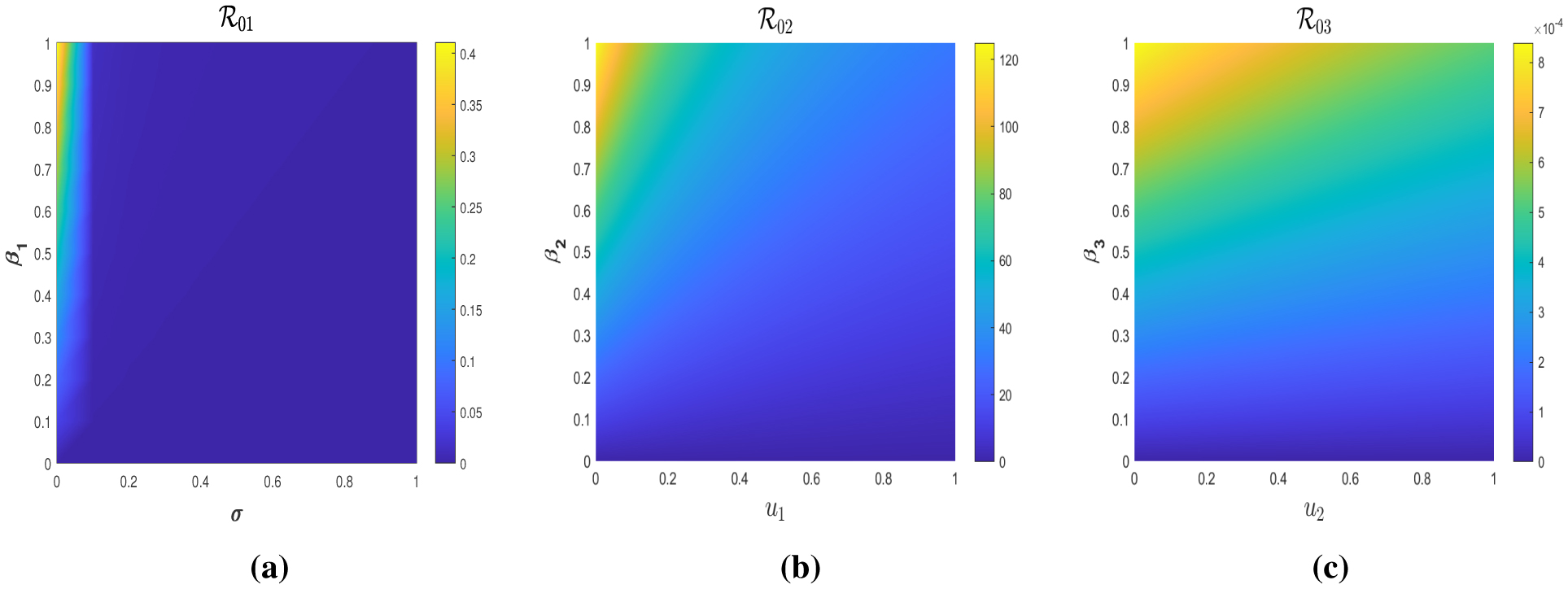
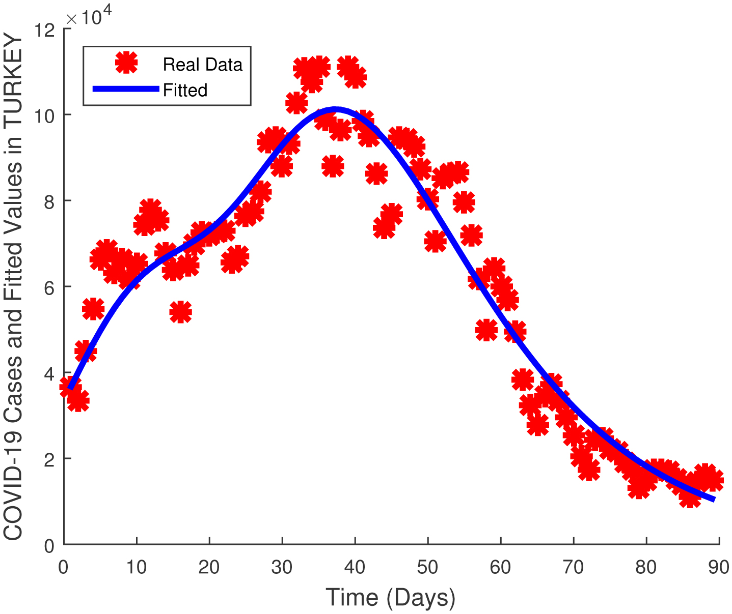
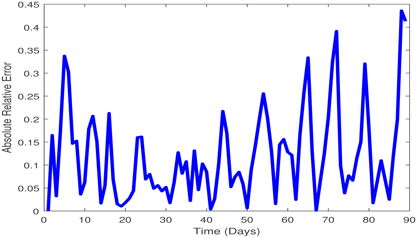
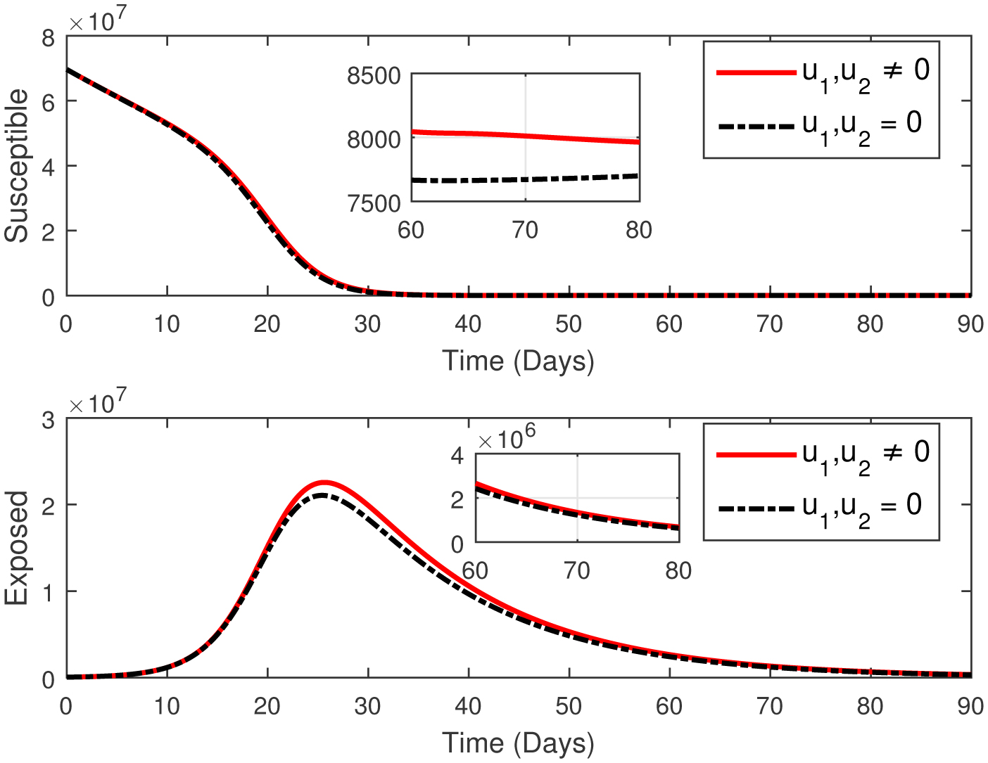
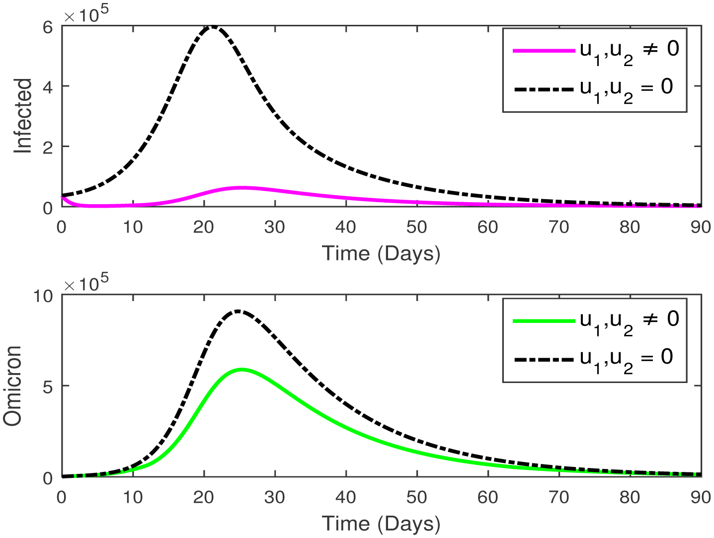
This paper presents an investigation into the relationship between heart attacks and the Omicron variant, employing a novel mathematical model. The model incorporates two adjustable control parameters to manage the number of infected individuals and individuals with the Omicron variant. The study examines the model's positivity and boundedness, evaluates the reproduction number (R₀), and conducts a sensitivity analysis of the control parameters based on the reproduction number. The model's parameters are estimated using the widely utilized least squares curve fitting method, employing real COVID-19 cases from Türkiye. Finally, numerical simulations demonstrate the efficacy of the suggested controls in reducing the number of infected individuals and the Omicron population.

Keywords:

Citation: Fırat Evirgen, Fatma Özköse, Mehmet Yavuz, Necati Özdemir. Real data-based optimal control strategies for assessing the impact of the Omicron variant on heart attacks[J]. AIMS Bioengineering, 2023, 10(3): 218-239. doi: 10.3934/bioeng.2023015

Related Papers:

[1]	Harman Kaur, Meenakshi Rana . Congruences for sixth order mock theta functions $\lambda(q)$ and $\rho(q)$ . Electronic Research Archive, 2021, 29(6): 4257-4268. doi: 10.3934/era.2021084
[2]	Meenakshi Rana, Shruti Sharma . Combinatorics of some fifth and sixth order mock theta functions. Electronic Research Archive, 2021, 29(1): 1803-1818. doi: 10.3934/era.2020092
[3]	Changjian Wang, Jiayue Zhu . Global dynamics to a quasilinear chemotaxis system under some critical parameter conditions. Electronic Research Archive, 2024, 32(3): 2180-2202. doi: 10.3934/era.2024099
[4]	Chang-Jian Wang, Yu-Tao Yang . Boundedness criteria for the quasilinear attraction-repulsion chemotaxis system with nonlinear signal production and logistic source. Electronic Research Archive, 2023, 31(1): 299-318. doi: 10.3934/era.2023015
[5]	Maoji Ri, Shuibo Huang, Canyun Huang . Non-existence of solutions to some degenerate coercivity elliptic equations involving measures data. Electronic Research Archive, 2020, 28(1): 165-182. doi: 10.3934/era.2020011
[6]	Nan Li . Summability in anisotropic mixed-norm Hardy spaces. Electronic Research Archive, 2022, 30(9): 3362-3376. doi: 10.3934/era.2022171
[7]	Lili Li, Boya Zhou, Huiqin Wei, Fengyan Wu . Analysis of a fourth-order compact $\theta$ -method for delay parabolic equations. Electronic Research Archive, 2024, 32(4): 2805-2823. doi: 10.3934/era.2024127
[8]	Jianxing Du, Xifeng Su . On the existence of solutions for the Frenkel-Kontorova models on quasi-crystals. Electronic Research Archive, 2021, 29(6): 4177-4198. doi: 10.3934/era.2021078
[9]	Zihan Zheng, Juan Wang, Liming Cai . Global boundedness in a Keller-Segel system with nonlinear indirect signal consumption mechanism. Electronic Research Archive, 2024, 32(8): 4796-4808. doi: 10.3934/era.2024219
[10]	Ying Hou, Liangyun Chen . Constructions of three kinds of Bihom-superalgebras. Electronic Research Archive, 2021, 29(6): 3741-3760. doi: 10.3934/era.2021059

Abstract

1. Introduction

Ramanujan's last letter to Hardy is one of the most mysterious and important mathematical letters in the history of mathematics. He introduced a class of functions that he called mock theta functions in his letter. For nearly a century, properties of these functions have been widely studied by different mathematicians. The important direction involves the arithmetic properties (see ^[1,2]), combinatorics (see ^[3,4]), identities between these functions, and generalized Lambert series (see ^[5,6]). For the interested reader, regarding the history and new developments in the study of mock theta functions, we refer to ^[7].

In 2007, McIntosh studied two second order mock theta functions in reference ^[8]; more details are given in reference ^[9]. These mock theta functions are:

$\begin{align} A(q) & = \sum\limits_{n = 0}^{\infty}\frac{q^{(n+1)^2}(-q;q^2)_n}{(q;q^2)_{(n+1)}^2} = \sum\limits_{n = 0}^{\infty}\frac{q^{n+1}(-q^2;q^2)_n}{(q;q^2)_{n+1}}, \end{align}$

(1.1)

$\begin{align} B(q)& = \sum\limits_{n = 0}^{\infty}\frac{q^n(-q;q^2)_n}{(q;q^2)_{n+1}} = \sum\limits_{n = 0}^{\infty}\frac{q^{n(n+1)}(-q^2;q^2)_n}{(q;q^2)_{n+1}^2}, \end{align}$

(1.2)

where

$(a;q)_n = \prod\limits_{i = 0}^{n-1}(1-aq^i),\;\; \; \; \; \; \; \; \; \; { }(a;q)_{\infty} = \prod\limits_{i = 0}^{\infty}(1-aq^i),$

$(a_1,a_2,\cdots,a_m;q)_{\infty} = (a_1;q)_{\infty}(a_2;q)_{\infty} \cdots (a_m;q)_{\infty},$

for $|q| < 1$ .

The functions $A(q)$ and $B(q)$ have been combinatorially interpreted in terms of overpartitions in ^[3] using the odd Ferrers diagram. In this paper, we study some arithmetic properties of one of the second order mock theta functions $B(q)$ . We start by noting, Bringmann, Ono and Rhoades ^[10] obtained the following identity:

$\begin{equation} \frac{B(q)+B(-q)}{2} = \frac{f_4^5}{f_2^4}, \end{equation}$

(1.3)

where

$f_m^k: = (q^m;q^m)_{\infty}^k,$

for positive integers $m$ and $k$ . We consider the function

$\begin{equation} B(q): = \sum\limits_{n = 0}^{\infty}b(n)q^n. \end{equation}$

(1.4)

Followed by Eq (1.3), the even part of $B(q)$ is given by:

$\begin{equation} \sum\limits_{n = 0}^{\infty}b(2n)q^n = \frac{f_2^5}{f_1^4}. \end{equation}$

(1.5)

In 2012, applying the theory of (mock) modular forms and Zwegers' results, Chan and Mao ^[5] established two identities for $b(n)$ , shown as:

$\begin{align} \sum\limits_{n = 0}^{\infty}b(4n+1)q^n & = 2\frac{f_2^8}{f_1^7}, \end{align}$

(1.6)

$\begin{align} \sum\limits_{n = 0}^{\infty}b(4n+2)q^n & = 4\frac{f_2^2f_4^4}{f_1^5}. \end{align}$

(1.7)

In a sequel, Qu, Wang and Yao ^[6] found that all the coefficients for odd powers of $q$ in $B(q)$ are even. Recently, Mao ^[11] gave analogues of Eqs (1.6) and (1.7) modulo 6

$\begin{align} \sum\limits_{n = 0}^{\infty}b({6n+2})q^n & = 4\frac{f_{2}^{10}f_{3}^{2}}{f_1^{10}f_6}, \end{align}$

(1.8)

$\begin{align} \sum\limits_{n = 0}^{\infty}b({6n+4})q^n & = 9\frac{f_{2}^4f_{3}^{4}f_{6}}{f_1^{8}}, \end{align}$

(1.9)

and proved several congruences for the coefficients of $B(q)$ . Motivated from this, we prove similar results for $b(n)$ by applying identities on the coefficients in arithmetic progressions. We present some congruence relations for the coefficients of $B(q)$ modulo certain numbers of the form $2^{\alpha}\cdot 3^{\beta}, 2^{\alpha}\cdot 5^{\beta}, 2^{\alpha}\cdot 7^{\beta}$ where $\alpha, \beta \geq 0.$ Our main theorems are given below:

Theorem 1.1. For $n \geq 0$ , we have

$\begin{align} \sum\limits_{n = 0}^{\infty}b(12n+9)q^n& = 18\left[\frac{f_2^9f_3^{12}}{f_1^{17}f_6^3}+2\frac{f_2^5f_3^4f_6}{f_1^9}+28\frac{f_2^6f_3^3f_6^6}{f_1^{14}}\right], \end{align}$

(1.10)

$\begin{align} \sum\limits_{n = 0}^{\infty}b(12n+10)q^n& = 36\left[2\frac{f_2^{16}f_6^{10}}{f_1^{20}f_3f_{12}^4}-q\frac{f_2^{28}f_3^3f_{12}^2}{f_1^{24}f_4^8f_6^2}-16q^2\frac{f_2^2f_3^3f_4^8f_{12}^2}{f_1^{16}f_6^2}\right]. \end{align}$

(1.11)

In particular, $b(12n+9)\equiv 0\pmod{18}, b(12n+10)\equiv 0\pmod{36}$ .

Theorem 1.2. For $n \geq 0$ , we have

$\begin{align} \sum\limits_{n = 0}^{\infty}b(18n+10)q^n& = 72\left[\frac{f_2^{16}f_3^{21}}{f_1^{27}f_6^9}+38q\frac{f_2^{13}f_3^{12}}{f_1^{24}}+64q^2\frac{f_2^{10}f_3^3f_6^9}{f_1^{21}}\right], \end{align}$

(1.12)

$\begin{align} \sum\limits_{n = 0}^{\infty}b(18n+16)q^n& = 72\left[5\frac{f_2^{15}f_3^{18}}{f_1^{26}f_6^6}+64q\frac{f_2^{12}f_3^9f_6^3}{f_1^{23}}+32q^2\frac{f_2^9f_6^{12}}{f_1^{20}}\right]. \end{align}$

(1.13)

In particular, $b(18n+10)\equiv 0\pmod{72}, b(18n+16)\equiv 0\pmod{72}.$

Apart from these congruences, we find some relations between $b(n)$ and restricted partition functions. Here we recall, Partition of a positive integer $\nu$ , is a representation of $\nu$ as a sum of non-increasing sequence of positive integers $\mu_1, \mu_2, \cdots, \mu_n$ . The number of partitions of $\nu$ is denoted by $p(\nu)$ which is called the partition function. If certain conditions are imposed on parts of the partition, is called the restricted partition and corresponding partition function is named as restricted partition function. Euler proved the following recurrence for $p(n)$ ^[12] [p. 12, Cor. 1.8]:

$\begin{array} p(n)-p(n-1)-p(n-2)+p(n-5)+p(n-7)-p(n-12)-p(n-15)+\cdots\\+(-1)^kp(n-k(3k-1)/2)+(-1)^kp(n-k(3k+1)/2)+\cdots = \begin{cases} 1, & \text { if } n = 0, \\ 0, & \text { otherwise. }\end{cases} \end{array}$

The numbers $k(3k\pm1)/2$ are pentagonal numbers. Following the same idea, different recurrence relations have been found by some researchers for restricted partition functions. For instance, Ewell ^[13] presented the recurrence for $p(n)$ involving the triangular numbers. For more study of recurrences, see ^[14,15,16]. Under the influence of these efforts, we express the coefficients of mock theta function $B(q)$ which are in arithmetic progression in terms of recurrence of some restricted partition functions.

This paper is organized as follows: Section 2, here we recall some preliminary lemmas and present the proof of Theorems 1.1 and 1.2. Section 3 includes some more congruences based on the above results. Section 4 depicts the links between $b(n)$ and some of the restricted partition functions.

2. Proof of Theorems 1.1 and 1.2

Before proving the results, we recall Ramanujan's theta function:

$j(a,b) = \sum\limits_{n = {-\infty}}^{\infty}a^{\frac{n(n+1)}{2}}b^{\frac{n(n-1)}{2}}, \text{ for} \; |ab| < 1.$

Some special cases of $j(a, b)$ are:

$\begin{align*} \phi(q)&: = j(q,q) = \sum\limits_{n = -\infty}^{\infty}q^{n^2} = \frac{f_2^5}{f_1^2f_4^2},\\ \psi(q)&: = j(q,q^3) = \sum\limits_{n = 0}^{\infty}q^{n(n+1)/2} = \frac{f_2^2}{f_1}. \end{align*}$

Also,

$\phi(-q) = \frac{f_1^2}{f_2}.$

The above function satisfy the following properties (see Entries 19, 20 in ^[17]).

$j(a,b) = (-a,-b,ab;ab)_{\infty}, \quad \text{(Jacobi's triple product identity)},$

$j(-q,-q^2) = (q;q)_{\infty}, \quad \text{(Euler's pentagonal number theorem)}.$

We note the following identities which will be used below.

Lemma 2.1. [^[18], Eq (3.1)] We have

$\begin{equation} \frac{f_2^3}{f_1^3} = \frac{f_6}{f_3}+3q\frac{f_6^4f_9^5}{f_3^8f_{18}}+6q^2\frac{f_6^3f_9^2f_{18}^2}{f_3^7}+12q^3\frac{f_6^2f_{18}^5}{f_3^6f_9}. \end{equation}$

(2.1)

Lemma 2.2. We have

$\begin{align} \frac{f_2^2}{f_1}& = \frac{f_6f_9^2}{f_3f_{18}}+q\frac{f_{18}^2}{f_9}, \end{align}$

(2.2)

$\begin{align} \frac{f_2}{f_1^2}& = \frac{f_6^4f_9^6}{f_3^8f_{18}^3}+2q\frac{f_6^3f_9^3}{f_3^7}+4q^2\frac{f_6^2f_{18}^3}{f_3^6}. \end{align}$

(2.3)

Proof. The first identity follows from [^[19] Eq (14.3.3)]. The proof of second identity can be seen from ^[20].

Lemma 2.3. We have

$\begin{align} \frac{1}{f_1^4}& = \frac{f_4^{14}}{f_2^{14}f_8^4}+4q\frac{f_4^2f_8^4}{f_2^{10}}, \end{align}$

(2.4)

$\begin{align} f_1^4& = \frac{f_4^{10}}{f_2^2f_8^4}-4q\frac{f_2^2f_8^4}{f_4^2}. \end{align}$

(2.5)

Proof. Identity (2.4) is Eq (1.10.1) from ^[19]. To obtain (2.5), replacing $q$ by $-q$ and then using

$(-q;-q)_{\infty} = \frac{f_2^3}{f_1f_4}.$

Now, we present the proof of Theorems 1.1 and 1.2.

Proof of Theorems 1.1 and 1.2. From Eq (1.6), we have

$\sum\limits_{n = 0}^{\infty}b(4n+1)q^n = 2\left(\frac{f_2^3}{f_1^3}\right)^3\cdot\frac{f_2^2}{f_1}.$

Substituting the values from Eqs (2.1) and (2.2) in above, we get

$\begin{eqnarray} \sum\limits_{n = 0}^{\infty}b(4n+1)q^n & = &2\frac{f_6^3f_9^2}{f_3^3f_{18}}+2q\frac{f_6^2f_{18}^2}{f_3^2f_9}+12q\frac{f_6^6f_9^7}{f_3^{10}f_{18}^2}+18q^2\frac{f_6^9f_9^{12}}{f_3^{17}f_{18}^3}+36q^2\frac{f_6^5f_9^4f_{18}}{f_3^9}+\\&&90q^3\frac{f_6^8f_9^9}{f_3^{16}}+72q^3\frac{f_6^4f_9f_{18}^4}{f_3^8}+48q^4\frac{f_6^3f_{18}^7}{f_3^7f_9^2}+288q^4\frac{f_6^7f_9^6f_{18}^3}{f_3^{15}}+\\&&504q^5\frac{f_6^6f_9^3f_{18}^6}{f_3^{14}}+576q^6\frac{f_6^5f_{18}^9}{f_3^{13}}. \end{eqnarray}$

(2.6)

Bringing out the terms involving $q^{3n+2}$ , dividing by $q^2$ and replacing $q^3$ by $q$ , we get (1.10). Considering Eq (1.5), we have

$\sum\limits_{n = 0}^{\infty}b(2n)q^n = \frac{f_2^3}{f_1^3}\cdot \frac{f_2^2}{f_1}.$

Substituting the values from Eqs (2.1) and (2.2), we obtain

$\begin{equation*} \sum\limits_{n = 0}^{\infty}b(2n)q^n = \left(\frac{f_6}{f_3}+3q\frac{f_6^4f_9^5}{f_3^8f_{18}}+6q^2\frac{f_6^3f_9^2f_{18}^2}{f_3^7}+12q^3\frac{f_6^2f_{18}^5}{f_3^6f_9}\right)\left(\frac{f_6f_9^2}{f_3f_{18}}+q\frac{f_{18}^2}{f_9}\right). \end{equation*}$

Extracting the terms involving $q^{3n}, q^{3n+1}, q^{3n+2}$ from the above equation, we have

$\begin{align} \sum\limits_{n = 0}^{\infty}b(6n)q^n& = \frac{f_2^2f_3^2}{f_1^2f_6}+18q\frac{f_2^3f_3f_6^4}{f_1^7}, \end{align}$

(2.7)

$\begin{align} \sum\limits_{n = 0}^{\infty}b(6n+2)q^n& = \frac{f_2f_6^2}{f_1f_3}+3\frac{f_2^5f_3^7}{f_1^9f_6^2}+12q\frac{f_2^2f_6^7}{f_1^6f_3^2}, \end{align}$

(2.8)

$\begin{align} \sum\limits_{n = 0}^{\infty}b(6n+4)q^n& = 9\frac{f_2^4f_3^4f_6}{f_1^8}. \end{align}$

(2.9)

Using Eqs (2.4) and (2.5) in Eq (2.9), we get

$\begin{equation*} \sum\limits_{n = 0}^{\infty}b(6n+4)q^n = 9f_2^4f_6\left(\frac{f_4^{14}}{f_2^{14}f_8^4}+4q\frac{f_4^2f_8^4}{f_2^{10}}\right)^2 \left(\frac{f_{12}^{10}}{f_6^2f_{24}^4}-4q^3\frac{f_6^2f_{24}^4}{f_{12}^2}\right). \end{equation*}$

Extracting the terms involving $q^{2n}, q^{2n+1}$ from above, we arrive at

$\begin{align} \sum\limits_{n = 0}^{\infty}b(12n+4)q^n& = 9\left(\frac{f_2^{28}f_6^{10}}{f_1^{24}f_3f_4^8f_{12}^4}+16q\frac{f_2^4f_4^8f_6^{10}}{f_1^{16}f_3f_{12}^4}-32q^2\frac{f_2^{16}f_3^3f_{12}^4}{f_1^{20}f_6^2}\right), \end{align}$

(2.10)

$\begin{align} \sum\limits_{n = 0}^{\infty}b(12n+10)q^n& = 9\left(8\frac{f_2^{16}f_6^{10}}{f_1^{20}f_3f_{12}^4}-4q\frac{f_2^{28}f_3^3f_{12}^4}{f_1^{24}f_4^8f_6^2}-16q^2\frac{f_2^4f_3^3f_4^8f_{12}^4}{f_1^{16}f_6^2}\right). \end{align}$

(2.11)

From Eq (2.11), we ultimately arrive at Eq (1.11). To prove Theorem 1.2, consider Eq (2.9) as:

$\begin{equation*} \sum\limits_{n = 0}^{\infty}b(6n+4)q^n = 9f_3^4f_6\left(\frac{f_2}{f_1^2}\right)^4. \end{equation*}$

Using Eq (2.3) in above, we get

$\begin{eqnarray} \sum\limits_{n = 0}^{\infty}b(6n+4)q^n& = &9\frac{f_6^{17}f_9^{24}}{f_3^{28}f_{18}^{12}}+72q\frac{f_6^{16}f_9^{21}}{f_3^{27}f_{18}^9}+360q^2\frac{f_6^{15}f_9^{18}}{f_3^{26}f_{18}^6}+288q^3\frac{f_6^{14}f_9^{15}}{f_3^{25}f_{18}^3}+\\&&864q^3\frac{f_6^{12}f_9^{15}}{f_3^{19}f_{18}^6}+2736q^4\frac{f_6^{13}f_9^{12}}{f_3^{24}}+4608q^5\frac{f_6^{12}f_{9}^{9}f_{18}^{3}}{f_{3}^{23}}+\\&&5760q^6\frac{f_{6}^{11}f_{9}^{6}f_{18}^{6}}{f_{3}^{22}}+4608q^7\frac{f_{6}^{10}f_{9}^{3}f_{18}^{9}}{f_{3}^{21}}+2304q^8\frac{f_{6}^{9}f_{18}^{12}}{f_{3}^{20}}. \end{eqnarray}$

(2.12)

Bringing out the terms involving $q^{3n+1}$ and $q^{3n+2}$ from Eq (2.12), we get Eqs (1.12) and (1.13), respectively.

3. Congruences

This segment of the paper contains some more interesting congruence relations for $b(n)$ .

Theorem 3.1. For $n \geq 0$ , we have

$\begin{align} b(12n+1) \equiv \begin{cases} 2(-1)^{k} \pmod 6, & \mathit{\text{if}}\; n = 3k(3 k+1)/2, \\ 0\pmod 6, & \mathit{\text{otherwise.}}\end{cases} \end{align}$

(3.1)

Theorem 3.2. For $n \geq 0$ , we have

$\begin{align} b(2n) \equiv \begin{cases} (-1)^{k}(2k+1) \pmod 4, & \mathit{\text{if}}\; n = k(k+1), \\ 0\pmod 4, & \mathit{\text{otherwise.}}\end{cases} \end{align}$

(3.2)

Theorem 3.3. For $n \geq 0$ , we have

$\begin{align} b(36n+10)& \equiv 0\pmod{72}, \end{align}$

(3.3)

$\begin{align} b(36n+13)& \equiv 0\pmod{6}, \end{align}$

(3.4)

$\begin{align} b(36n+25)& \equiv 0\pmod{12}, \end{align}$

(3.5)

$\begin{align} b(36n+34)& \equiv 0\pmod{144}, \end{align}$

(3.6)

$\begin{align} b(108n+t)& \equiv 0\pmod{18},\; \; \mathit{\text{for t}} \in \{49,85\}. \end{align}$

(3.7)

Theorem 3.4. For $n \geq 0$ , we have

$\begin{align} b(20n+t)& \equiv 0\pmod{5},\; \; \mathit{\text{for t}} \in \{8,16\} \end{align}$

(3.8)

$\begin{align} b(20n+t)& \equiv 0\pmod{20}, \; \; \mathit{\text{for t}} \in \{6,18\} \end{align}$

(3.9)

$\begin{align} b(20n+17)& \equiv 0\pmod{10}, \end{align}$

(3.10)

$\begin{align} b(28n+t)& \equiv 0\pmod{14},\; \; \mathit{\text{for t}} \in \{5,21,25\}. \end{align}$

(3.11)

Proof of Theorem 3.1. From Eq (2.6), picking out the terms involving $q^{3n}$ and replacing $q^3$ by $q$ , we have

$\begin{align} \sum\limits_{n = 0}^{\infty} b(12 n+1) q^{n} = 2 \frac{f_{2}^{3} f_{3}^{2}}{f_{1}^{3} f_{6}}+90 q \frac{f_{2}^{8} f_{3}^{9}}{f_{1}^{16}}+72 q \frac{f_{2}^{4} f_{3} f_{6}^{4}}{f_{1}^{8}}+576 q^{2} \frac{f_{2}^{5} f_{6}^{9}}{f_{1}^{3}}. \end{align}$

(3.12)

Reducing modulo 6, we obtain

$\begin{align} \sum\limits_{n = 0}^{\infty} b(12n+1) q^{n} \equiv 2f_3 \pmod 6. \end{align}$

(3.13)

With the help of Euler's pentagonal number theorem,

$\begin{align*} \sum\limits_{n = 0}^{\infty} b(12 n+1) q^{n} \equiv 2\sum\limits_{k = -\infty}^{\infty}(-1)^kq^{\frac{3k(3k+1)}{2}} \pmod 6, \end{align*}$

which completes the proof of Theorem 3.1.

Proof of Theorem 3.2. Reducing Eq (1.5) modulo 4, we get

$\begin{equation} \sum\limits_{n = 0}^{\infty}b(2n)q^n\equiv f_2^3 \pmod 4. \end{equation}$

(3.14)

From Jacobi's triple product identity, we obtain

$\begin{equation*} \sum\limits_{n = 0}^{\infty}b(2n)q^n\equiv \sum\limits_{k = 0}^{\infty}(-1)^k(2k+1)q^{k(k+1)} \pmod 4, \end{equation*}$

which completes the proof of Theorem 3.2.

Proof of Theorem 3.3. Consider Eq (1.11), reducing modulo 72

$\begin{equation*} \sum\limits_{n = 0}^{\infty}b(12n+10)q^n \equiv 36q \frac{f_{2}^{28}f_{3}^{3}f_{12}^{4}}{f_{1}^{24}f_{4}^{8}f_{6}^{2}} \pmod{72}, \end{equation*}$

$\begin{align*} \sum\limits_{n = 0}^{\infty}b(12n+10)q^n& \equiv 36q\frac{f_{2}^{28}f_{3}^{3}f_{12}^{4}}{f_{2}^{12}f_{4}^{8}f_{12}} = 36q\frac{f_{2}^{16}f_{3}^{3}f_{12}^3}{f_{4}^{8}}\pmod{72} \end{align*}$

$\begin{equation} \sum\limits_{n = 0}^{\infty}b(12n+10)q^n \equiv 36qf_3^3f_{12}^3\pmod{72}. \end{equation}$

(3.15)

Extracting the terms involving $q^{3n}$ , replacing $q^3$ by $q$ in Eq (3.15), we arrive at Eq (3.3). Similarly, consider Eq (1.13) and reducing modulo 144, we have

$\begin{align*} \sum\limits_{n = 0}^{\infty}b(18n+16)q^n & \equiv 72\cdot5\frac{f_{2}^{15}f_{3}^{18}}{f_{1}^{26}f_{6}^{6}}\pmod{144},\\ &\equiv72\frac{f_{2}^{15}f_{6}^{9}}{f_{2}^{13}f_{6}^{6}} = 72f_{2}^{2}f_{6}^{3}\pmod{144}. \end{align*}$

Extracting the terms involving $q^{2n+1}$ , dividing both sides by $q$ and replacing $q^2$ by $q$ , we get Eq (3.6).

From Eq (3.20), we get

$\begin{align*} \sum\limits_{n = 0}^{\infty}b(12n+1)q^n & \equiv 2f_3 \pmod6. \end{align*}$

Bringing out the terms containing $q^{3n+1}$ , dividing both sides by $q$ and replacing $q^3$ by $q$ , we have $b(36n+13) \equiv 0 \pmod6.$ Reducing Eq (3.12) modulo 12, we have

$\begin{equation*} \sum\limits_{n = 0}^{\infty}b(12n+1)q^n \equiv 2\frac{f_2^3f_3^2}{f_1^3f_{6}}+90q\frac{f_2^8f_3^9}{f_1^{16}}\pmod{12}, \end{equation*}$

$\begin{equation*} \sum\limits_{n = 0}^{\infty}b(12n+1)q^n \equiv 2\frac{f_3^2}{f_{6}}\left(\frac{f_6}{f_3}+3q\frac{f_6^4f_9^5}{f_3^8f_{18}}+6q^2\frac{f_6^3f_9^2f_{18}^2}{f_3^7}+12q^3\frac{f_6^2f_{18}^5}{f_3^6f_9}\right)+6q\frac{f_2^8f_3^9}{f_2^{8}}. \end{equation*}$

Extracting the terms containing $q^{3n+2}$ , dividing by $q^2$ and replacing $q^3$ by $q$ , we obtain Eq (3.5). Reducing Eq (3.12) modulo 18,

$\begin{align*} \sum\limits_{n = 0}^{\infty}b(12n+1)q^n &\equiv 2\frac{f_2^3f_3^2}{f_1^3f_{6}}\pmod{18},\\ & = 2\frac{f_3^2}{f_{6}}\left(\frac{f_6}{f_3}+3q\frac{f_6^4f_9^5}{f_3^8f_{18}}+6q^2\frac{f_6^3f_9^2f_{18}^2}{f_3^7}+12q^3\frac{f_6^2f_{18}^5}{f_3^6f_9}\right). \end{align*}$

Extracting the terms involving $q^{3n+1}$ , dividing both sides by $q$ and replacing $q^3$ by $q$ , we have

$\sum\limits_{n = 0}^{\infty}b(36n+13)q^n \equiv 6\frac{f_2^3f_3^5}{f_1^6f_6} \equiv 6\frac{f_6f_3^5}{f_3^2f_6}\pmod{18}$

$\sum\limits_{n = 0}^{\infty}b(36n+13)q^n \equiv 6f_3^3\pmod{18}.$

Extracting the terms containing $q^{3n+1}, q^{3n+2}$ from above to get Eq (3.7).

Proof of Theorem 3.4. From Eqs (1.5) and (2.4), we have

$\begin{equation*} \sum\limits_{n = 0}^{\infty}b(2n)q^n = f_2^5\left(\frac{f_4^{14}}{f_2^{14}f_8^4}+4q\frac{f_4^2f_8^4}{f_2^{10}}\right). \end{equation*}$

Bringing out the terms containing even powers of $q$ , we obtain

$\begin{equation*} \sum\limits_{n = 0}^{\infty}b(4n)q^n = \frac{f_2^{14}}{f_1^9f_4^4}, \end{equation*}$

which can be written as:

$\begin{equation*} \sum\limits_{n = 0}^{\infty}b(4n)q^n = \frac{f_2^{15}}{f_1^{10}f_4^5}.\frac{f_1f_4}{f_2} \equiv \frac{f_{10}^3}{f_5^2f_{20}}.\frac{f_1f_4}{f_2}\pmod{5}. \end{equation*}$

Here

$\begin{align*} \frac{f_1f_4}{f_2}& = \frac{(q;q)_{\infty}(q^4;q^4)_{\infty}}{(q^2;q^2)_{\infty}},\\ & = \frac{(q;q^2)_{\infty}(q^2;q^2)_{\infty}(q^4;q^4)_{\infty}}{(q^2;q^2)_{\infty}}, \end{align*}$

$\begin{equation} \frac{f_1f_4}{f_2} = (q,q^3,q^4;q^4)_{\infty} = \sum\limits_{n = {-\infty}}^{\infty}(-1)^nq^{2n^2-n}, \end{equation}$

(3.16)

where the last equality follows from Jacobi's triple product identity. Using the above identity, we have

$\begin{equation} \sum\limits_{n = 0}^{\infty}b(4n)q^n \equiv \frac{f_{10}^3}{f_5^2f_{20}}\sum\limits_{n = {-\infty}}^{\infty}(-1)^nq^{2n^2-n}\pmod{5}. \end{equation}$

(3.17)

Since ${2n^2-n} \not\equiv 2, 4\pmod5$ , it follows that the coefficients of $q^{5n+2}, q^{5n+4}$ in $\sum_{n = 0}^{\infty}b(4n)q^n$ are congruent to $0\pmod5$ , which proves that $b(20n+t)\equiv 0\pmod5$ , for $t \in \{8, 16\}$ .

Consider Eq (1.7)

$\begin{equation*} \sum\limits_{n = 0}^{\infty}b(4n+2)q^n = 4\frac{f_4^5}{f_1^5}\frac{f_2^2}{f_4}\equiv 4\frac{f_{20}}{f_5}\frac{f_2^2}{f_4}\pmod{20}. \end{equation*}$

Now

$\begin{align*} \frac{f_2^2}{f_4}& = \frac{(q^2;q^2)_{\infty}^2}{(q^4;q^4)_{\infty}},\\ & = \frac{(q^2;q^2)_{\infty}(q^2;q^4)_{\infty}(q^4;q^4)_{\infty}}{(q^4;q^4)_{\infty}}, \end{align*}$

$\frac{f_2^2}{f_4} = (q^2,q^2,q^4;q^4)_{\infty} = \sum\limits_{n = {-\infty}}^{\infty}(-1)^nq^{2n^2}.$

Using the above identity, we get

$\begin{equation} \sum\limits_{n = 0}^{\infty}b(4n+2)q^n\equiv 4\frac{f_{20}}{f_5}\sum\limits_{n = {-\infty}}^{\infty}(-1)^nq^{2n^2}\pmod{20}. \end{equation}$

(3.18)

Since ${2n^2} \not\equiv 1, 4\pmod5$ , it follows that the coefficients of $q^{5n+1}, q^{5n+4}$ in $\sum_{n = 0}^{\infty}b(4n+2)q^n$ are congruent to $0\pmod{20}$ , which proves Eq (3.9). For the proof of next part, consider Eq (1.6) as:

$\begin{equation*} \sum\limits_{n = 0}^{\infty}b(4n+1)q^n = 2\frac{f_2^5}{f_1^{10}}{f_1^3}{f_2^3} \equiv 2\frac{f_{10}}{f_{5}^2}f_1^3f_2^3\pmod{10}, \end{equation*}$

$\begin{equation} \sum\limits_{n = 0}^{\infty}b(4n+1)q^n\equiv 2\frac{f_{10}}{f_{5}^2}\sum\limits_{k = 0}^{\infty}(-1)^k(2k+1)q^{\frac{k(k+1)}{2}}\sum\limits_{m = 0}^{\infty}(-1)^m (2m+1)q^{m(m+1)}\pmod{10}. \end{equation}$

(3.19)

Therefore, to contribute the coefficient of $q^{5n+4}$ , $(k, m)\equiv (2, 2)\pmod5$ and thus the contribution towards the coefficient of $q^{5n+4}$ is a multiple of 5.

Consider Eq (1.6) as:

$\begin{equation*} \sum\limits_{n = 0}^{\infty}b(4n+1)q^n = 2\frac{f_2^7}{f_1^7}f_2 \equiv 2\frac{f_{14}}{f_{7}}f_2\pmod{14}. \end{equation*}$

With the help of Euler's pentagonal number theorem,

$\begin{equation} \sum\limits_{n = 0}^{\infty}b(4n+1)q^n \equiv 2\frac{f_{14}}{f_{7}}\sum\limits_{n = {-\infty}}^{\infty}(-1)^nq^{n(3n+1)}\pmod{14}. \end{equation}$

(3.20)

As ${n(3n+1)}\not\equiv 1, 5, 6\pmod7$ , it readily proves Eq (3.11).

4. Recurrence relations

In this section, we find some recurrence relations connecting $b(n)$ and restricted partition functions. First we define some notations. Let $\overline{p}_l(n)$ denotes the number of overpartitions of $n$ with $l$ copies. Then

$\sum\limits_{n = 0}^{\infty}\overline{p}_l(n)q^n = \left(\frac{f_2}{f_1^2}\right)^l.$

Let $p_{ld}(n)$ denotes the number of partitions of $n$ into distinct parts with $l$ copies. Then

$\sum\limits_{n = 0}^{\infty}p_{ld}(n)q^n = \left(\frac{f_2}{f_1}\right)^l.$

Theorem 4.1. We have

$\begin{align} b(2n)& = \overline{p}_2(n)-3\overline{p}_2(n)+5\overline{p}_2(n)+\cdots+(-1)^k(2k+1)\overline{p}_2(n-k(k+1))+\cdots,{ \quad } \end{align}$

(4.1)

$\begin{array} b(2n) = p_{4d}(n)-p_{4d}(n-2)-p_{4d}(n-4)+p_{4d}(n-10)+p_{4d}(n-14)+\cdots+\\ (-1)^kp_{4d}(n-{k(3k-1)})+(-1)^kp_{4d}(n-{k(3k+1)})+\cdots. \end{array}$

(4.2)

Theorem 4.2.

$\begin{array} b(4n+1) = 2p_{8d}(n)-2p_{8d}(n-1)-2p_{8d}(n-2)+2p_{8d}(n-5)+2p_{8d}(n-7)+ \cdots+\\ (-1)^k2p_{8d}\left(n-\frac{k(3k-1)}{2}\right)+(-1)^k2p_{8d}\left(n-\frac{k(3k+1)}{2}\right)+\cdots, \end{array}$

(4.3)

$\begin{equation} b(4n+1) = 2\sum\limits_{c = 0}^{n}b(2c)p_{3d}(n-c). \quad \end{equation}$

(4.4)

Theorem 4.3.

$\begin{array} b(6n+2) = 4p_{10d}(n)-8p_{10d}(n-3)+8p_{10d}(n-12)+8p_{10d}(n-27)+\cdots\\ +8(-1)^kp_{10d}(n-3k^2)+\cdots. \end{array}$

(4.5)

Proof of Theorem 4.1. Consider (1.5) as:

$\begin{equation*} \sum\limits_{n = 0}^{\infty}b(2n)q^n = \left(\frac{f_2}{f_1^2}\right)^2\cdot f_2^3. \end{equation*}$

Then

$\begin{align*} \sum\limits_{n = 0}^{\infty}b(2n)q^n& = \left(\sum\limits_{n = 0}^{\infty}\overline{p}_2(n)q^n\right)\left(\sum\limits_{k = 0}^{\infty}(-1)^k(2k+1)q^{k(k+1)}\right),\\ & = \sum\limits_{n = 0}^{\infty}\sum\limits_{k = 0}^{\infty}(-1)^k(2k+1)\overline{p}_2(n)q^{n+k(k+1)},\\ & = \sum\limits_{n = 0}^{\infty}\left(\sum\limits_{k = 0}^{\infty}(-1)^k(2k+1)\overline{p}_2(n-k(k+1))\right)q^n. \end{align*}$

From the last equality, we readily arrive at (4.1). To prove (4.2), consider (1.5) as:

$\begin{align*} \sum\limits_{n = 0}^{\infty}b(2n)q^n& = \left(\frac{f_{2}}{f_{1}}\right)^4\cdot{f_2},\\ & = \left(\sum\limits_{n = 0}^{\infty}p_{4d}(n)q^n\right)\left(\sum\limits_{k = -\infty}^{\infty}(-1)^kq^{k(3k+1)}\right),\\ & = \left(\sum\limits_{n = 0}^{\infty}p_{4d}(n)q^n\right)\left(1+\sum\limits_{k = 1}^{\infty}(-1)^kq^{k(3k-1)}+\sum\limits_{k = 1}^{\infty}(-1)^kq^{k(3k+1)}\right), \end{align*}$

$\begin{align*}\sum\limits_{n = 0}^{\infty}b(2n)q^n = \sum\limits_{n = 0}^{\infty}p_{4d}(n)q^n+\sum\limits_{n = 0}^{\infty}\left(\sum\limits_{k = 1}^{\infty}(-1)^kp_{4d}(n)q^{k(3k-1)+n}\right)+\sum\limits_{n = 0}^{\infty}\left(\sum\limits_{k = 1}^{\infty}(-1)^kp_{4d}(n)q^{k(3k+1)+n}\right), \end{align*}$

$\begin{align*} \sum\limits_{n = 0}^{\infty}b(2n)q^n = \sum\limits_{n = 0}^{\infty}p_{4d}(n)q^n+\sum\limits_{n = 0}^{\infty}\left(\sum\limits_{k = 1}^{\infty}(-1)^kp_{4d}(n-k(3k-1))q^{n}\right)\\+\sum\limits_{n = 0}^{\infty}\left(\sum\limits_{k = 1}^{\infty}(-1)^kp_{4d}(n-k(3k+1))q^{n}\right), \end{align*}$

which proves Eq (4.2).

Proof of Theorem 4.2. Consider Eq (1.6) as:

$\begin{align*} \sum\limits_{n = 0}^{\infty}b(4n+1)q^n& = 2\left(\frac{f_2}{f_1}\right)^8{f_1},\\ & = 2\left(\sum\limits_{n = 0}^{\infty}p_{8d}(n)q^n\right)\left(\sum\limits_{k = -\infty}^{\infty}(-1)^kq^{\frac{k(3k+1)}{2}}\right),\\ & = 2\left(\sum\limits_{n = 0}^{\infty}p_{8d}(n)q^n\right)\left(1+\sum\limits_{k = 1}^{\infty}(-1)^kq^{k(3k-1)/2}+\sum\limits_{k = 1}^{\infty}(-1)^kq^{k(3k+1)/2}\right), \end{align*}$

$\begin{align*} \sum\limits_{n = 0}^{\infty}b(4n+1)q^n = \sum\limits_{n = 0}^{\infty}p_{8d}(n)q^n+\sum\limits_{n = 0}^{\infty}\sum\limits_{k = 1}^{\infty}(-1)^kp_{8d}(n)q^{k(3k-1)/2+n}+\sum\limits_{n = 0}^{\infty}\sum\limits_{k = 1}^{\infty}(-1)^kp_{8d}(n)q^{k(3k+1)/2+n}, \end{align*}$

$\begin{align*} \sum\limits_{n = 0}^{\infty}b(4n+1)q^n = \sum\limits_{n = 0}^{\infty}p_{8d}(n)q^n+\sum\limits_{n = 0}^{\infty}\left(\sum\limits_{k = 1}^{\infty}(-1)^kp_{8d}\left(n-\frac{k(3k-1)}{2}\right)\right)q^{n}\\+\sum\limits_{n = 0}^{\infty}\left(\sum\limits_{k = 1}^{\infty}(-1)^kp_{8d}\left(n-\frac{k(3k+1)}{2}\right)\right)q^{n}, \end{align*}$

which proves Eq (4.3). To prove Eq (4.4), consider Eq (1.6) as:

$\begin{align*} \sum\limits_{n = 0}^{\infty}b(4n+1)q^n& = 2\left(\frac{f_2^5}{f_1^4}\right)\frac{f_2^3}{f_1^3},\\ & = 2\left(\sum\limits_{n = 0}^{\infty}b(2n)q^n\right)\left(\sum\limits_{k = 0}^{\infty}p_{3d}(k)q^k\right),\\ & = 2\sum\limits_{n = 0}^{\infty}\left(\sum\limits_{c = 0}^{n}b(2c)p_{3d}(n-c)\right)q^n. \end{align*}$

Comparing the coefficients of $q^{n}$ , we arrive at Eq (4.4).

Proof of Theorem 4.3. Consider Eq (1.8) as:

$\begin{align*} \sum\limits_{n = 0}^{\infty}b(6n+2)q^n& = 4\left(\frac{f_2}{f_1}\right)^{10}\cdot \frac{f_3^2}{f_6},\\ & = 4\left(\sum\limits_{n = 0}^{\infty}p_{10d}(n)q^n\right)\left(\sum\limits_{k = -\infty}^{\infty}(-1)^kq^{3k^2}\right),\\ & = 4\left(\sum\limits_{n = 0}^{\infty}p_{10d}(n)q^n\right)\left(1+2\sum\limits_{k = 1}^{\infty}(-1)^kq^{3k^2}\right),\\ & = 4\sum\limits_{n = 0}^{\infty}p_{10d}(n)q^n+8\sum\limits_{n = 0}^{\infty}\left(\sum\limits_{k = 1}^{\infty}(-1)^kp_{10d}(n)q^{3k^2+n}\right),\\ & = 4\sum\limits_{n = 0}^{\infty}p_{10d}(n)q^n+8\sum\limits_{n = 0}^{\infty}\left(\sum\limits_{k = 1}^{\infty}(-1)^kp_{10d}(n-3k^2)\right) q^{n}. \end{align*}$

Comparing the coefficients of $q^n$ to obtain Eq (4.5).

5. Conclusion and open problems

In this paper, we have provided the arithmetic properties of second order mock theta function $B(q)$ , introduced by McIntosh. Some congruences are proved for the coefficients of $B(q)$ modulo specific numbers. The questions which arise from this work are:

(i) Are there exist congruences modulo higher primes for $B(q)$ ?

(ii) Is there exist any other technique (like modular forms) that helps to look for some more arithmetic properties of $B(q)$ ?

(iii) How can we explore the other second order mock theta function $A(q)$ ?

Acknowledgments

The first author is supported by University Grants Commission (UGC), under grant Ref No. 971/(CSIR-UGC NET JUNE 2018) and the the second author is supported by Science and Engineering Research Research Board (SERB-MATRICS) grant MTR/2019/000123. The authors of this paper are thankful to Dr. Rupam Barman, IIT Guwahati, for his valuable insight during establishing Theorems 3.1 and 3.2. We would like to thank the referee for carefully reading our paper and offering corrections and helpful suggestions.

Conflict of interest

The authors declare there is no conflicts of interest.

References

[1]	Mishra P, Parveen R, Bajpai R, et al. (2021) Impact of cardiovascular diseases on severity of COVID-19 patients: a systematic review. Ann Acad Med Singap 50: 52-60. https://doi.org/10.47102/annals-acadmedsg.2020367
[2]	Harrison SL, Buckley BJ, Rivera-Caravaca JM, et al. (2021) Cardiovascular risk factors, cardiovascular disease, and COVID-19: an umbrella review of systematic reviews. Eur Heart J-Qual Car 7: 330-339. https://doi.org/10.1093/ehjqcco/qcab029
[3]	Clerkin KJ, Fried JA, Raikhelkar J, et al. (2021) COVID-19 and cardiovascular disease. Circulation 141: 1648-1655. https://doi.org/10.1161/CIRCULATIONAHA.120.046941
[4]	Naik PA, Eskandari Z, Yavuz M, et al. (2022) Complex dynamics of a discrete-time Bazykin-Berezovskaya prey-predator model with a strong Allee effect. J Comput Appl Math 413: 114401. https://doi.org/10.1016/j.cam.2022.114401
[5]	Sene N (2022) Second-grade fluid with Newtonian heating under Caputo fractional derivative: analytical investigations via Laplace transforms. Math Model Num Simul Appl 2: 13-25. https://doi.org/10.53391/mmnsa.2022.01.002
[6]	Sabbar Y (2023) Asymptotic extinction and persistence of a perturbed epidemic model with different intervention measures and standard lévy jumps. Bull Biomath 1: 58-77. https://doi.org/10.59292/bulletinbiomath.2023004
[7]	Hammouch Z, Yavuz M, Özdemir N (2021) Numerical solutions and synchronization of a variable-order fractional chaotic system. Math Model Num Simul Appl 1: 11-23. https://doi.org/10.53391/mmnsa.2021.01.002
[8]	Naik PA, Yavuz M, Qureshi S, et al. (2020) Modeling and analysis of COVID-19 epidemics with treatment in fractional derivatives using real data from Pakistan. Eur Phys J Plus 135: 1-42. https://doi.org/10.1140/epjp/s13360-020-00819-5
[9]	Joshi H, Yavuz M, Townley S, et al. (2023) Stability analysis of a non-singular fractional-order covid-19 model with nonlinear incidence and treatment rate. Phys Scripta 98: 045216. https://doi.org/10.1088/1402-4896/acbe7a
[10]	Atede AO, Omame A, Inyama SC (2023) A fractional order vaccination model for COVID-19 incorporating environmental transmission: a case study using Nigerian data. Bull Biomath 1: 78-110. https://doi.org/10.59292/bulletinbiomath.2023005
[11]	Uçar S, Uçar E, Özdemir N, et al. (2019) Mathematical analysis and numerical simulation for a smoking model with Atangana–Baleanu derivative. Chaos Soliton Fract 118: 300-306. https://doi.org/10.1016/j.chaos.2018.12.003
[12]	Naik PA, Owolabi KM, Yavuz M, et al. (2020) Chaotic dynamics of a fractional order HIV-1 model involving AIDS-related cancer cells. Chaos Soliton Fract 140: 110272. https://doi.org/10.1016/j.chaos.2020.110272
[13]	Evirgen F, Ucar E, Ucar S, et al. (2023) Modelling influenza a disease dynamics under Caputo-Fabrizio fractional derivative with distinct contact rates. Math Model Num Simul Appl 3: 58-72. https://doi.org/10.53391/mmnsa.1274004
[14]	Uçar E, Uçar S, Evirgen F, et al. (2021) A fractional SAIDR model in the frame of Atangana–Baleanu derivative. Fractal Fract 5: 32. https://doi.org/10.3390/fractalfract5020032
[15]	Elhia M, Balatif O, Boujallal L, et al. (2021) Optimal control problem for a tuberculosis model with multiple infectious compartments and time delays. IJOCTA 11: 75-91. https://doi.org/10.11121/ijocta.01.2021.00885
[16]	Nwajeri UK, Atede AO, Panle AB, et al. (2023) Malaria and cholera co-dynamic model analysis furnished with fractional-order differential equations. Math Model Num Simul Appl 3: 33-57. https://doi.org/10.53391/mmnsa.1273982
[17]	Agarwal P, Nieto JJ, Torres DFM (2022) Mathematical Analysis of Infectious Diseases. Academic Press. https://doi.org/10.1016/C2020-0-03443-2
[18]	Yıldız TA, Arshad S, Baleanu D (2018) New observations on optimal cancer treatments for a fractional tumor growth model with and without singular kernel. Chaos Soliton Fract 117: 226-239. https://doi.org/10.1016/j.chaos.2018.10.029
[19]	Malinzi J, Ouifki R, Eladdadi A, et al. (2018) Enhancement of chemotherapy using oncolytic virotherapy: Mathematical and optimal control analysis. Math Biosci Eng 15: 1435-1463. https://doi.org/10.3934/mbe.2018066
[20]	Yıldız TA (2019) A comparison of some control strategies for a non-integer order tuberculosis model. IJOCTA 9: 21-30. https://doi.org/10.11121/ijocta.01.2019.00657
[21]	Yıldız TA, Karaoğlu E (2019) Optimal control strategies for tuberculosis dynamics with exogenous reinfections in case of treatment at home and treatment in hospital. Nonlinear Dynam 97: 2643-2659. https://doi.org/10.1007/s11071-019-05153-9
[22]	Baleanu D, Jajarmi A, Sajjadi SS, et al. (2019) A new fractional model and optimal control of a tumor-immune surveillance with non-singular derivative operator. Chaos 29: 083127. https://doi.org/10.1063/1.5096159
[23]	Abidemi A, Aziz NAB (2020) Optimal control strategies for dengue fever spread in Johor, Malaysia. Comput Meth Prog Bio 196: 105585. https://doi.org/10.1016/j.cmpb.2020.105585
[24]	Jajarmi A, Yusuf A, Baleanu D, et al. (2020) A new fractional HRSV model and its optimal control: a non-singular operator approach. Physica A 547: 123860. https://doi.org/10.1016/j.physa.2019.123860
[25]	Naik PA, Zu J, Owolabi KM (2020) Global dynamics of a fractional order model for the transmission of HIV epidemic with optimal control. Chaos Soliton Fract 138: 109826. https://doi.org/10.1016/j.chaos.2020.109826
[26]	Ameen I, Baleanu D, Ali HM (2020) An efficient algorithm for solving the fractional optimal control of SIRV epidemic model with a combination of vaccination and treatment. Chaos Soliton Fract 137: 109892. https://doi.org/10.1016/j.chaos.2020.109892
[27]	Elhia M, Balatif O, Boujallal L, et al. (2021) Optimal control problem for a tuberculosis model with multiple infectious compartments and time delays. IJOCTA 11: 75-91. https://doi.org/10.11121/ijocta.01.2021.00885
[28]	Sweilam NH, Al-Mekhlafi SM, Albalawi AO, et al. (2021) Optimal control of variable-order fractional model for delay cancer treatments. Appl Math Model 89: 1557-1574. https://doi.org/10.1016/j.apm.2020.08.012
[29]	Zhao J, Yang R (2021) A dynamical model of echinococcosis with optimal control and cost-effectiveness. Nonlinear Anal Real World Appl 62: 103388. https://doi.org/10.1016/j.nonrwa.2021.103388
[30]	Mohammadi H, Kumar S, Rezapour S, et al. (2021) A theoretical study of the Caputo–Fabrizio fractional modeling for hearing loss due to Mumps virus with optimal control. Chaos Soliton Fract 144: 110668. https://doi.org/10.1016/j.chaos.2021.110668
[31]	Abbasi Z, Zamani I, Mehra AHA, et al. (2020) Optimal control design of impulsive SQEIAR epidemic models with application to COVID-19. Chaos Soliton Fract 139: 110054. https://doi.org/10.1016/j.chaos.2020.110054
[32]	Moussouni N, Aliane M (2021) Optimal control of COVID-19. IJOCTA 11: 114-122. https://doi.org/10.11121/ijocta.01.2021.00974
[33]	Nabi KN, Kumar P, Erturk VS (2021) Projections and fractional dynamics of COVID-19 with optimal control strategies. Chaos Soliton Fract 145: 110689. https://doi.org/10.1016/j.chaos.2021.110689
[34]	Arruda EF, Das SS, Dias CM, et al. (2021) Modelling and optimal control of multi strain epidemics, with application to COVID-19. Plos One 16: e0257512. https://doi.org/10.1371/journal.pone.0257512
[35]	Tchoumi SY, Diagne ML, Rwezaura H, et al. (2021) Malaria and COVID-19 co-dynamics: A mathematical model and optimal control. Appl Math Model 99: 294-327. https://doi.org/10.1016/j.apm.2021.06.016
[36]	Araz SI (2021) Analysis of a Covid-19 model: optimal control, stability and simulations. Alexandria Eng J 60: 647-658. https://doi.org/10.1016/j.aej.2020.09.058
[37]	Rosa S, Torres DFM (2022) Fractional modelling and optimal control of COVID-19 transmission in Portugal. Axioms 11: 170. https://doi.org/10.3390/axioms11040170
[38]	Fatima B, Yavuz M, ur Rahman M, et al. (2023) Modeling the epidemic trend of middle eastern respiratory syndrome coronavirus with optimal control. Math Biosc Eng 20: 11847-11874. https://doi.org/10.3934/mbe.2023527
[39]	Özköse F, Yavuz M (2022) Investigation of interactions between COVID-19 and diabetes with hereditary traits using real data: a case study in Turkey. Comput Biol Med 141: 105044. https://doi.org/10.1016/j.compbiomed.2021.105044
[40]	Driessche VP, Watmough J (2002) Reproduction numbers and sub-threshold endemic equilibria for compartmental models of disease transmission. Math Biosci 180: 29-48. https://doi.org/10.1016/S0025-5564(02)00108-6
[41]	Diekmann O, Heesterbeek JAP, Roberts MG (2010) The construction of next-generation matrices for compartmental epidemic models. J R Soc Interface 7: 873-885. https://doi.org/10.1098/rsif.2009.0386
[42]	Chitnis N, Hyman JM, Cushing JM (2008) Determining important parameters in the spread of malaria through the sensitivity analysis of a mathematical model. Bull Math Biol 70: 1272. https://doi.org/10.1007/s11538-008-9299-0
[43]	Coddington EA, Levinson N Theory of Ordinary Differential Equations (1955). Tata McGraw-Hill Education
[44]	Gaff HD, Schaefer E, Lenhart S (2011) Use of optimal control models to predict treatment time for managing tick-borne disease. J Biol Dynam 5: 517-530. https://doi.org/10.1080/17513758.2010.535910
[45]	. Pontryagin LS (1987) Mathematical Theory of Optimal Processes, 1 Ed., CRC Press. https://doi.org/10.1201/9780203749319
[46]	. Lenhart S, Workman JT (2007) Optimal Control Applied to Biological Models, 1 Ed., CRC Press. https://doi.org/10.1201/9781420011418
[47]	Vitiello A, Ferrara F, Auti AM, et al. (2022) Advances in the Omicron variant development. J Int Med 292: 81-90. https://doi.org/10.1111/joim.13478

This article has been cited by:

1.	Olivia X.M. Yao, New congruences modulo 9 for the coefficients of Gordon-McIntosh's mock theta function ξ ( q ) , 2024, 47, 1607-3606, 239, 10.2989/16073606.2023.2205604
2.	Yueya Hu, Eric H. Liu, Olivia X. M. Yao, Congruences modulo 4 and 8 for Ramanujan’s sixth-order mock theta function $\rho (q)$ , 2025, 66, 1382-4090, 10.1007/s11139-024-01018-x

Reader Comments

Your name:*

Email:*
© 2023 the Author(s), licensee AIMS Press. This is an open access article distributed under the terms of the Creative Commons Attribution License (http://creativecommons.org/licenses/by/4.0)