
Citation: Todd Lael Siler. Neurotranslations: Interpreting the Human Brain’s Attention System[J]. AIMS Medical Science, 2016, 3(2): 179-202. doi: 10.3934/medsci.2016.2.179
[1] | ZongWang, Qimin Zhang, Xining Li . Markovian switching for near-optimal control of a stochastic SIV epidemic model. Mathematical Biosciences and Engineering, 2019, 16(3): 1348-1375. doi: 10.3934/mbe.2019066 |
[2] | Xuehui Ji, Sanling Yuan, Tonghua Zhang, Huaiping Zhu . Stochastic modeling of algal bloom dynamics with delayed nutrient recycling. Mathematical Biosciences and Engineering, 2019, 16(1): 1-24. doi: 10.3934/mbe.2019001 |
[3] | Dongmei Li, Tana Guo, Yajing Xu . The effects of impulsive toxicant input on a single-species population in a small polluted environment. Mathematical Biosciences and Engineering, 2019, 16(6): 8179-8194. doi: 10.3934/mbe.2019413 |
[4] | Linda J. S. Allen, P. van den Driessche . Stochastic epidemic models with a backward bifurcation. Mathematical Biosciences and Engineering, 2006, 3(3): 445-458. doi: 10.3934/mbe.2006.3.445 |
[5] | Zeyan Yue, Sheng Wang . Dynamics of a stochastic hybrid delay food chain model with jumps in an impulsive polluted environment. Mathematical Biosciences and Engineering, 2024, 21(1): 186-213. doi: 10.3934/mbe.2024009 |
[6] | An Ma, Shuting Lyu, Qimin Zhang . Stationary distribution and optimal control of a stochastic population model in a polluted environment. Mathematical Biosciences and Engineering, 2022, 19(11): 11260-11280. doi: 10.3934/mbe.2022525 |
[7] | Maoxiang Wang, Fenglan Hu, Meng Xu, Zhipeng Qiu . Keep, break and breakout in food chains with two and three species. Mathematical Biosciences and Engineering, 2021, 18(1): 817-836. doi: 10.3934/mbe.2021043 |
[8] | Dawid Czapla, Sander C. Hille, Katarzyna Horbacz, Hanna Wojewódka-Ściążko . Continuous dependence of an invariant measure on the jump rate of a piecewise-deterministic Markov process. Mathematical Biosciences and Engineering, 2020, 17(2): 1059-1073. doi: 10.3934/mbe.2020056 |
[9] | H.Thomas Banks, Shuhua Hu . Nonlinear stochastic Markov processes and modeling uncertainty in populations. Mathematical Biosciences and Engineering, 2012, 9(1): 1-25. doi: 10.3934/mbe.2012.9.1 |
[10] | Linard Hoessly, Carsten Wiuf . Fast reactions with non-interacting species in stochastic reaction networks. Mathematical Biosciences and Engineering, 2022, 19(3): 2720-2749. doi: 10.3934/mbe.2022124 |
With the rapid development of industry and agriculture, the environment pollution has caused many serious ecological problems (see [1,2,3]), such as the reduction of species diversity and the extinction of some species. Therefore, it motivates many scholars' interest to study dynamic behavior of population in a polluted environment by establishing mathematical models. The population model in a polluted environment was first proposed by Hallam et al.[4,5]. From then on, more investigations and discussions on the dynamic behavior of the deterministic population model can be found (see [6,7,8,9,10]). But in practical problems, population changes are affected not only by environmental noise but also by sudden changes of temperature and climate. Thus, several scholars have introduced random perturbations into population model to study dynamic behavior. For example, Liu and Wang [11] established the stochastic population model with impulsive toxicant input and obtained sufficient conditions on extinction, persistence, stability in the mean. Subsequently, Yu et al. [12] proved the existence of global positive solution for the stochastic population model with Allee effect under regime switching and established the threshold. In [13], Wei et al. proposed a stochastic population model with partial tolerance, discussed the conditions for population the extinction and proved the stationary distribution with ergodicity by constructing the Lyapunov function. Liu et al. [14] considered the significance of white noise and color noise on population persistence and extinction and studied stochastic population model with Markov switching. More research results on the persistence, extinction, and stability of random population models and others have been presented (see [15,16,17,18,19]). However, the above mentioned references didn't consider the invariant measure of population system with diffusion.
In fact, in the real world, the population and toxins in the ecology spread around the medium such as soil and water. In addition, we also know that the existence and uniqueness of invariant measure is one of the important properties for stochastic population model with Markov switching and diffusion. Nevertheless, if we introduce diffusion into stochastic population model, the corresponding Kolmogorov-Fokker-Planck (KFP) equation will become more complicated. Furthermore, the invariant measure of stochastic population model with Markov switching and diffusion is difficult to obtain. Therefore, it is of great significance to choose an effective numerical approximation method. To the best of our knowledge, the explicit Euler-Maruyama (EM) method has the advantages of easy calculation and small calculation amount. Motivated by [21,20], in the paper, we first develop a new stochastic population model with Markov switching and diffusion. Under suitable regularity assumptions, we discuss the existence and uniqueness of numerical invariant measure generated by the EM method. Subsequently, we prove that numerical invariant measure converges to the invariant measure of exact solution in the Wasserstein distance sense. In particular, the main contributions of the paper are as follows:
● We establish a novel stochastic population model with diffusion and Markov switching in a polluted environment. By using the Chebyshev's inequality, we obtain the existence and uniqueness of invariant measure for the model.
● Under local Lipschitz conditions, we study the approximation of numerical invariant measure generated by the EM method for the newly developed model.
The structure of this article is as follows: In Section2, we introduce some necessary preliminary knowledge results for the following analysis. In Section3, based on the Perron-Frobenius theorem, we study existence and uniqueness of invariant measure for the exact solution. In Section4, we mainly study the existence and uniqueness of numerical invariant measure for the EM scheme. In addition, we also prove that the numerical invariant measure of the EM scheme converges to invariant measure of exact solution. In Section5, the numerical example is given to verify our theoretical results. In Section6, we give the conclusions of this study.
In this paper, we introduce Markov switching and spatial diffusion into the model mentioned by Liu and Wang [15], and obtain the following model
{dX1(t,x)=[k1(t,x)ΔX1(t,x)+β(t,x,X2(t,x),Λt)X1(t,x)]dt−μ(t,x,X2(t,x),Λt)X1(t,x)dt+g(t,X1(t,x),Λt)dWt,in(0,T)×Γ,dX2(t,x)=[k2(t,x)ΔX2(t,x)+K(Λt)X3(t,x)−(l(Λt)+m(Λt))X2(t,x)]dt,in(0,T)×Γ,dX3(t,x)=[k3(t,x)ΔX3(t,x)−M(Λt)X3(t,x)+u(t,x)]dt,in(0,T)×Γ,X1(0,x)=s1(x),X2(0,x)=s2(x),X3(0,x)=s3(x),inx∈Γ,X1(t,x)=0,X2(t,x)=0,X3(t,x)=0,on(0,T]×∂Γ, | (2.1) |
where L:=(0,T)×Γ, Γ is a bounded domain in R3 with smooth boundary ∂Γ, t∈(0,T); X1(t,x) denotes the population density at the location x at time t. X2(t,x) is the concentration of toxicant in the organism at time t and in spatial position x. The concentration of toxicant in the environment at the location x at time t is described by X3(t,x). K(Λt) is the net organismal uptake rate of toxicant from the environment at time t. M(Λt) is the total loss rate of the toxicant from the environment. μ(t,x,X2(t,x),Λt) denotes the decreasing rate function of the population at time t and in spatial position x. ki>0,i=1,2,3 is the diffusion coefficient. β(t,x,X2(t,x),Λt) describes the intrinsic growth rate function of the population at time t and in spatial position x. u(t,x) denotes the exogenous total toxicant input into environment at time t and in spatial position x. l(Λt) is the net organismal excretion rate of toxicant and m(Λt) is depuration rate of toxicant due to metabolic process and other losses.
Throughout the paper, Let (V,‖⋅‖) and (H,|⋅|) be two separable Hilbert spaces, with norm denoted by ‖⋅‖ and |⋅|, respectively. V is viewed as a subspace of H with a continuous dense embedding. V⋐H represents the embedding is compact. V′ and H′ are the dual of V, H. We set H3:=H×H×H. Let (Ω,F,P) be a complete probability space with {Ft}0≤t≤T the natural filtration generated by the Brownian motion Wt, which means Ft=σ{Ws;0≤s≤t} augmented with all P-null sets of F0. To construct such a filtration, we denote by N the collection of P-null sets, i.e. N={B∈F:P(B)=0}. In the paper, C>0 represents different positive constants. Let Λt, t>0, be a right-continuous Markov chain on the probability space taking values in a finite state S={1,2,…,N} for some positive integer N<∞. The generator of {Λt}t>0 is specified by Q=(qij)N×N, such that for a sufficiently small Δ,
P(Λt+Δ=j|Λt=i)={qijΔ+o(Δ),i≠j,1+qiiΔ+o(Δ),i=j, | (2.2) |
where Δ>0, o(Δ) satisfies limΔ→0o(Δ)Δ=0. Here qij is the transition rate from i to j satisfying qii=−∑i≠jqij. We assume that the Markov chain {Λt} defined on the probability space above is independent of the standard Brownian motion {Wt}t≥0 and the Q matrix is irreducible and conservative. Therefore, the Markov chain {Λt}t≥0 has a unique stationary distribution π:=(π1,…,πN) which can be determined by solving the linear equation
πQ=0subjecttoN∑i=1πi=1withπi>0. |
Let P(H3×S) stand for the family of all probability measures on H3×S. For ξ=(ξ1,ξ2,ξ3)∗∈H3, ξ≫0 means each component ξi>0, i=1,2,3.
Next, let's give some necessary assumptions:
(H1) Setting Xsk,ik,t:=Xsk,ik(t,x), k=1,2,3, there exists a positive constant ρi such that for i∈S, (t,x)∈L
‖g(t,Xs1,i1,t,i)−g(t,Xˉs1,i1,t,i)‖2≤ρi|Xs1,i1,t−Xˉs1,i1,t|2, | (2.3) |
where s1 and ˉs1 are the different initial values of the first equation for system (2.1).
From (H1), for each i∈S and Xs1,i1,t∈H, we can obtain that for (t,x)∈L
‖g(t,Xs1,i1,t,i)‖2≤C+ρi|Xs1,i1,t|2, | (2.4) |
where C depends on the initial value of the function g(t,Xs1,i1,t,i).
(H2) For each i∈S, there exist positive constants ˉM, ˉβ and ˉμ such that
{ˉM:=maxi{M(Λi)},0<ˉM<∞;0≤β(t,x,Xs2,i2,t,Λi)≤ˉβ<∞;0≤μ0≤μ(t,x,Xs2,i2,t,Λi)≤ˉμ<∞. | (2.5) |
(H3) u(t,x) is non-negative measurable in L, there exists a positive constant ˉu such that
0≤u0≤u(t,x)≤ˉu<∞. | (2.6) |
We replace ((X1,t,X2,t,X3,t),Λt) with ((Xs1,i1,t,Xs2,i2,t,Xs3,i3,t),Λit), especially the initial value
((X01,X02,X03),Λ0)=((s1,s2,s3),i). |
For any p∈(0,1], we set s:=(s1,s2,s3) and define a metric on H3×S as follows
dp((s,i),(ˉs,i)):=∫H33∑k=1|sk−ˉsk|p+I{i≠j},(s,i),(ˉs,i)∈H3×S, |
where IA denotes the indicator function of the set A, and ˉs:=(ˉs1,ˉs2,ˉs3) is different initial value. For p∈(0,1], we define the Wassertein distance between ν∈P(H3×S) and ν′∈P(H3×S) by
Wp(ν,ν′)=infEdp(Xk,Xk′), |
where the infimum is taken over all pairs of random variables Xk, Xk′ on H3×S with respective laws ν, ν′. Let Pt((s1,s2,s3),i;⋅) be the transition probability kernel of the pair ((Xs1,i1,t,Xs2,i2,t,Xs3,i3,t),Λit), a time homogeneous Markov process (see [22]). Recall that π∈P(H3×S) is called an invariant measure of ((Xs1,i1,t,Xs2,i2,t,Xs3,i3,t),Λit) if
π(A×{i})=N∑j=1∫H3Pt((s1,s2,s3),j;A×{i})π(d(s1,s2,s3)×{j}),t≥0,A∈H3,i∈S | (2.7) |
holds. For any p>0, let
diag(ρ)≜diag(ρ1,…,ρN),Qp≜Q+p2diag(ρ),ηp≜−maxγReγ. | (2.8) |
where ρi is introduced in the assumptions and γ∈spec(Qp), spec(Qp) denotes the spectrum of Qp(i.e., the multi-set of its eigenvalues). Reγ is the real part of γ and diag(ρ1,…,ρN) denotes the diagonal matrix whose diagonal entries are ρ1,…,ρN, respectively.
In this section, we mainly prove the existence and uniqueness of the invariant measure for the exact solution, under the assumption conditions (H1)–(H3). Firstly, in order to prove the existence and uniqueness of the underlying invariant measure, we prepare the following lemma.
Lemma 3.1. (see [22]) Let N<∞ and assume further that
N∑i=1μiρi<0, | (3.1) |
where μi is the stationary distribution of Markov chain {Λt}t≥0, and ρi is introduced in the assumption (H1). Then
(1) ηp>0 if maxi∈Sρi≤0;
(2) ηp>0 for p<maxi∈S,ρi>0{−2qii/ρi} if maxi∈Sρi>0.
Remark 1: The system (2.1) is said to be attractive " in average " if Eq (3.1) holds. The Lemma 3.1 provides great convenience to study the existence and uniqueness of invariant measure for exact solution, i.e., the proof of Theorem 3.1.
Theorem 3.1. Let N<∞ and assume further that (H1)–(H3) hold with maxi∈Sρi>0. Then the exact solution of system (2.1) admits a unique invariant measure π∈P(H3×S).
Proof. The key point of proof is to divide the whole proof into two parts of existence and uniqueness.
(I) Existence of invariant measure. Let ((Ys1,i1,t,Ys2,i2,t,Ys3,i3,t),Λit) be the exact solution of system (2.1) with ((s1,s2,s3),i) as initial value, where ((s1,s2,s3),i)∈H3×S. A simple application of the Feynman-Kac formula show that let Qp,t=etQp, where Qp is given in Eq (2.8). Then, the spectral radius Ria(Qp,t) (i.e., Ria(Qp,t)=supλ∈spec(Qp,t)|λ|) of Qp,t equals to e−ηpt. Since all coefficients of Qp,t are positive, by the Perron-Frobenius theorem (see [23]) yields that −ηp is a simple eigenvalue of Qp, all other eigenvalues have a strictly smaller real part. Note that the eigenvector of Qp,t corresponding to e−ηpt is also an eigenvector of Qp corresponding to −ηp. According to Perron-Frobenius theorem, for Qp it can be found that there is a positive eigenvector ξ(p)=(ξ(p)1,…,ξ(p)N)≫0 corresponding to the eigenvalue −ηp, and ξ(p)≫0 means that each component ξ(p)i>0. Let
p0=1∧mini∈S,ρi>0{−2qii/ρi}, | (3.2) |
where 1∧mini∈S,ρi>0{−2qii/ρi}:=min{1,mini∈S,ρi>0{−2qii/ρi}}. Combined with Lemma 3.1, we can get
Qpξ(p)i=−ηpξ(p)i≪0. | (3.3) |
In order to investigate the existence and uniqueness of invariant measure for exact solution, we need to prove the boundedness of exact solution for system (2.1). In other words, we need to prove whether the following inequality holds.
E(1+|Ys1,i1,t|p+|Ys2,i2,t|p+|Ys3,i3,t|p)≤C. |
First, using the Itˆo's formula (see [24], Theorem 1.45 of p.48), we can have
eηptE((1+|Ys1,i1,t|2+|Ys2,i2,t|2+|Ys3,i3,t|2)p/2ξ(p)Λit)=(1+|s1|2+|s2|2+|s3|2)p2ξpi+E∫t0eηpϵ(1+|Ys1,i1,ϵ|2+|Ys2,i2,ϵ|2+|Ys3,i3,ϵ|2)p2{ηpξ(p)Λiϵ+(Qξ(p))(Λiϵ)}dϵ+p2E∫t0eηpϵ(1+|Ys1,i1,ϵ|2+|Ys2,i2,ϵ|2+|Ys3,i3,ϵ|2)p2−1ξ(p)Λiϵ{2⟨Ys2,i2,ϵ,K(Λiϵ)Ys3,i3,ϵ−(l(Λiϵ)+m(Λiϵ))Ys2,i2,ϵ⟩+2⟨Ys1,i1,ϵ,k1ΔYs1,i1,ϵ+βYs1,i1,ϵ−μYs1,i1,ϵ⟩+2⟨Ys3,i3,ϵ,−M(Λiϵ)Ys3,i3,ϵ+uϵ+k3ΔYs3,i3,ϵ⟩+2⟨Ys2,i2,ϵ,k2ΔYs2,i2,ϵ⟩}dϵ+p2∫t0eηpϵE(1+|Ys1,i1,ϵ|2+|Ys2,i2,ϵ|2+|Ys3,i3,ϵ|2)p2−1×ξ(p)Λiϵ{(p−2)(1+|Ys1,i1,ϵ|2+|Ys2,i2,ϵ|2+|Ys3,i3,ϵ|2)−1‖Ys1,i1,ϵ∗g(ϵ,Ys1,i1,ϵ,Λiϵ)‖2+‖g(ϵ,Ys1,i1,ϵ,Λiϵ)‖2}dϵ. |
Using p(p−2)/2<0, due to p∈(0,p0), and combining with the following inequality,
∫t0∫Ωk(t,x)ΔYk,ϵYk,ϵdxdϵ=−∫t0∫Ωk(t,x)▽Yk,ϵ▽Yk,ϵdxdϵ≤−k0∫t0‖Yk,ϵ‖2dϵ,k=1,2,3 | (3.4) |
where 0≤k0≤k(t,x)<∞ (k0 is a constant). Further, we have
eηptE((1+|Ys1,i1,t|2+|Ys2,i2,t|2+|Ys3,i3,t|2)p/2ξ(p)Λit)≤(1+|s1|2+|s2|2+|s3|2)p2ξ(p)i+p2E∫t0eηpϵ(1+|Ys1,i1,ϵ|2+|Ys2,i2,ϵ|2+|Ys3,i3,ϵ|2)p2−1{2⟨Ys1,i1,ϵ,βYs1,i1,ϵ−μYs1,i1,ϵ⟩+ε1(K(Λiϵ))2|Ys2,i2,ϵ|2+1ε1|Ys3,i3,ϵ|2+2(l(Λiϵ)+m(Λiϵ))|Ys2,i2,ϵ|2+ε2|Ys3,i3,ϵ|2+1ε2|uϵ|2+2ˉM|Ys3,i3,ϵ|2}ξ(p)Λiϵdϵ+p2∫t0eηpϵE(1+|Ys1,i1,ϵ|2+|Ys2,i2,ϵ|2+|Ys3,i3,ϵ|2)p2−1‖g(s,Ys1,i1,ϵ,Λiϵ)‖2ξ(p)Λiϵdϵ+E∫t0eηpϵ(1+|Ys1,i1,ϵ|2+|Ys2,i2,ϵ|2+|Ys3,i3,ϵ|2)p2{ηpξ(p)Λiϵ+(Qξ(P))(Λiϵ)}dϵ. |
Therefore, based on assumption conditions (H1)–(H3) and the inequality 2ab≤εa2+1εb2, ε>0 we can obtain
eηptE((1+|Ys1,i1,t|2+|Ys2,i2,t|2+|Ys3,i3,t|2)p/2ξ(p)Λit)≤(1+|s1|2+|s2|2+|s3|2)p2ξ(p)i+p2E∫t0eηpϵ(1+|Ys1,i1,ϵ|2+|Ys2,i2,ϵ|2+|Ys3,i3,ϵ|2)p2−1{c+[2(ˉβ−μ0)+ρΛiϵ]|Ys1,i1,ϵ|2+[2(l(Λiϵ)+m(Λiϵ))+ε1ˉK2]|Ys2,i2,ϵ|2+[2ˉM+1ε2+1ε1]|Ys3,i3,ϵ|2+ε2|uϵ|2}dϵ+E∫t0eηpϵ(1+|Ys1,i1,ϵ|2+|Ys2,i2,ϵ|2+|Ys3,i3,ϵ|2)p2{ηpξ(p)Λiϵ+(Qξ(P))(Λiϵ)}dϵ, |
where ˉK:=maxi{K(Λi)}, for all i∈S, 0<ˉK<∞. Then, setting C1:=2(ˉβ−μ0)+ρ0, ρ0:=maxi∈S|ρΛiϵ| C2:=maxi∈S2(l(Λiϵ)+m(Λiϵ))+ε1ˉK2 and C3:=2ˉM+1ε2+1ε1, C4:=ε2+c are different constants and using the inequality
(|a|+|b|)r≤2r−1(|a|r+|b|r),r≥1,∀a,b∈R, | (3.5) |
we can further estimate
eηptE((1+|Ys1,i1,t|2+|Ys2,i2,t|2+|Ys3,i3,t|2)p/2ξ(p)Λit)≤c(1+|s1|p+|s2|p+|s3|p)+E∫t0eηpϵ(1+|Ys1,i1,ϵ|2+|Ys2,i2,ϵ|2+|Ys3,i3,ϵ|2)p2{ηpξ(p)Λis+(Qξ(P))(Λiϵ)}dϵ+p2E∫t0eηpϵ(1+|Ys1,i1,ϵ|2+|Ys2,i2,ϵ|2+|Ys3,i3,ϵ|2)p2{C1|Ys1,i1,ϵ|2+C2|Ys2,i2,ϵ|2(1+|Ys1,i1,ϵ|2+|Ys2,i2,ϵ|2+|Ys3,i3,ϵ|2)}dϵ+p2E∫t0eηpϵ(1+|Ys1,i1,ϵ|2+|Ys2,i2,ϵ|2+|Ys3,i3,ϵ|2)p2{C3|Ys3,i3,ϵ|2+C4|uϵ|2(1+|Ys1,i1,ϵ|2+|Ys2,i2,ϵ|2+|Ys3,i3,ϵ|2)}dϵ. |
Finally, by the Gronwall's lemma, we can get the result
eηptE((1+|Ys1,i1,t|2+|Ys2,i2,t|2+|Ys3,i3,t|2)p/2ξ(p)Λit)≤CeCT, | (3.6) |
and further estimates can be obtained as follows
supt≥0E((|Ys1,i1,t|p+|Ys2,i2,t|p+|Ys3,i3,t|p)≤C. | (3.7) |
For ∀ t>0, we can define a probability measure
χt(A)=1t∫t0Pϵ(s,i;A)dϵ,A∈(H3×S). |
Then, let Ys,it:=(Ys1,i1,t,Ys2,i2,t,Ys3,i3,t), for any ε>0, by Eq (3.7) and Chebyshev's inequality, there exists an r>0 sufficiently large such that
χt(Kr×S)=1t∫t0Pϵ(s,i;Kr×S)dϵ≥1−supt≥0(E|Ys,it|p)rp≥1−ε. | (3.8) |
Hence, χt is tight since the compact embedding V⋐H, then Kr={s∈H3;|s|≤r} is a compact subset of H3 (see [25], Definition 2, p.27) for each i∈S. Combined with the Fellerian property of transition seimgroup for Pt(s,i;⋅) and according to Krylov-Bogoliubov theorem (see [26]), ((Ys1,i1,t,Ys2,i2,t,Ys3,i3,t),Λit) has an invariant measure (see [27]). Next, we prove the uniqueness of the invariant measure for ((Ys1,i1,t,Ys2,i2,t,Ys3,i3,t),Λit).
(II) Uniqueness of invariant measure. First, let ((Ys1,i1,t,Ys2,i2,t,Ys3,i3,t),Λit) and ((Yˉs1,i1,t,Yˉs2,i2,t,Yˉs3,i3,t),Λit) be the solutions of the system (2.1) satisfying the initial values ((s1,s2,s3),i) and ((ˉs1,ˉs2,ˉs3),i), respectively. Under assumption conditions (H1)–(H3), we take ∀ε∈(0,1) and use Itˆo's formula, combined with Eq (3.4), we have
eηptE((ε+|Ys1,i1,t−Yˉs1,i1,t|2+|Ys2,i2,t−Yˉs2,i2,t|2+|Ys3,i3,t−Yˉs3,i3,t|2)p/2ξ(p)Λit)≤(ε+|s1−ˉs1|2+|s2−ˉs2|2|+|s3−ˉs3|2|)p/2ξ(p)i+p2E∫t0eηpϵ(ε+|Ys1,i1,ϵ−Yˉs1,i1,ϵ|2+|Ys2,i2,ϵ−Yˉs2,i2,ϵ|2+|Ys3,i3,ϵ−Yˉs3,i3,ϵ|2)p/2−1ξ(p)Λiϵ×{[2(ˉβ−μ0)+ρΛiϵ]|Ys1,i1,ϵ−Yˉs1,i1,ϵ|2+ε1ˉK2|Ys2,i2,ϵ−Yˉs2,i2,ϵ|2+[1ε1+1ε2+2ˉM]|Ys3,i3,ϵ−Yˉs3,i3,ϵ|2+2(l(Λiϵ)+m(Λiϵ))|Ys2,i2,ϵ−Yˉs2,i2,ϵ|2+ε2|us3,iϵ−uˉs3,iϵ|2}dϵ≤(ε+|s1−ˉs1|2+|s2−ˉs2|2|+|s3−ˉs3|2)p/2ξ(p)i+p2E∫t0eηpϵ(ε+|Ys1,i1,ϵ−Yˉs1,i1,ϵ|2+|Ys2,i2,ϵ−Yˉs2,i2,ϵ|2+|Ys3,i3,ϵ−Yˉs3,i3,ϵ|2)p/2ξ(p)Λiϵ×{C1|Ys1,i1,ϵ−Yˉs1,i1,ϵ|2+C2|Ys2,i2,ϵ−Yˉs2,i2,ϵ|2+C3|Ys3,i3,ϵ−Yˉs3,i3,ϵ|2+ε2|us3,iϵ−uˉs3,iϵ|2ε+|Ys1,i1,ϵ−Yˉs1,i1,ϵ|2+|Xs2,i2,ϵ−Xˉs2,i2,ϵ|2+|Xs3,i3,ϵ−Xˉs3,i3,ϵ|2}dϵ, |
where Ci, i=1,2,3 have been explained before and ρΛiϵ is introduced in the assumption (H1). In addition, using the result of Eqs (3.5) and (3.6), we can get
eηptE((ε+|Ys1,i1,t−Yˉs1,i1,t|2+|Ys2,i2,t−Yˉs2,i2,t|2+|Ys3,i3,t−Xˉs3,i3,t|2)p/2ξ(p)Λit)≤(ε+|s1−ˉs1|2+|s2−ˉs2|2+|s3−ˉs3|2)p/2ξ(p)i+p2CE∫t0eηpϵ(ε+|Ys1,i1,ϵ−Yˉs1,i1,ϵ|2+|Ys2,i2,ϵ−Xˉs2,i2,ϵ|2+|Xs3,i3,ϵ−Xˉs3,i3,ϵ|2)p/2ξ(p)Λiϵ×{1−ε(ε+|Ys1,i1,ϵ−Yˉs1,i1,ϵ|2+|Ys2,i2,ϵ−Yˉs2,i2,ϵ|2+|Xs3,i3,ϵ−Xˉs3,i3,ϵ|2)−1}dϵ≤(ε+|s1−ˉs1|2+|s2−ˉs2|2|+|s3−ˉs3|2)p/2ξ(p)i+Cεp/2eηpt, | (3.9) |
when ε→0, we can get the following result
E(|Ys1,i1,t−Yˉs1,i1,t|p+|Ys2,i2,t−Yˉs2,i2,t|p+|Ys3,i3,t−Yˉs3,i3,t|p)≤C(|s1−ˉs1|p+|s2−ˉs2|p+|s3−ˉs3|p)e−ηpt. | (3.10) |
Define the stopping time
τ=inf{t≥0:Λit=Λjt}. |
According to the definition of S and irreducibility of Q, there exists θ>0 such that
P(τ>t)≤e−θt,t>0. | (3.11) |
Due to p∈(0,p0), and choose q>1 such that 0<pq<p0, where p0 is introduced in Eq (3.2). Using H¨older's inequality, we can have
E(|Ys1,i1,t−Yˉs1,j1,t|p+|Ys2,i2,t−Yˉs2,j2,t|p+|Ys3,i3,t−Yˉs3,j3,t|p)=E(|Ys1,i1,t−Yˉs1,j1,t|p1{τ>t/2})+E(|Ys1,i1,t−Yˉs1,j1,t|p1{τ≤t/2})+E(|Ys2,i2,t−Yˉs2,j2,t|p1{τ>t/2})+E(|Ys2,i2,t−Yˉs2,j2,t|p1{τ≤t/2})+E(|Ys3,i3,t−Yˉs3,j3,t|p1{τ>t/2})+E(|Ys3,i3,t−Yˉs3,j3,t|p1{τ≤t/2})≤(E|Ys1,i1,t−Yˉs1,j1,t|pq1{τ>t/2})1/q(P(τ>t/2))1/p+E(1{τ≤t/2}E|YYs1,i1,τ,Λiτ1,t−τ−YYˉs1,j1,τ,Λjτ1,t−τ|p)+(E|Ys2,i2,t−Yˉs2,j2,t|pq1{τ>t/2})1/q(P(τ>t/2))1/p+E(1{τ≤t/2}E|YYs2,i2,τ,Λiτ2,t−τ−YYˉs2,j2,τ,Λjτ2,t−τ|p)+(E|Ys3,i3,t−Yˉs1,j3,t|pq1{τ>t/2})1/q(P(τ>t/2))1/p+E(1{τ≤t/2}E|YYs3,i3,τ,Λiτ3,t−τ−YYˉs3,j1,τ,Λjτ3,t−τ|p). | (3.12) |
Applying the result of Eq (3.11), we further obtain
\begin{equation} \begin{split} &\mathbb{E}(|Y_{1, t}^{s_{1}, i}-Y_{1, t}^{\bar{s}_{1}, j}|^{p}+|Y_{2, t}^{s_{2}, i}-Y_{2, t}^{\bar{s}_{2}, j}|^{p}+|Y_{3, t}^{s_{3}, i}-Y_{3, t}^{\bar{s}_{3}, j}|^{p})\\ \leq&e^{-\frac{q-1}{2q}\theta t}(\mathbb{E}|Y_{1, t}^{s_{1}, i}-Y_{1, t}^{\bar{s}_{1}, j}|^{pq})^{\frac{1}{q}}+C\mathbb{E}({\mathbf1}_{\{\tau\leq t/2\}}e^{-\eta_{p}(t-\tau)}\mathbb{E}|Y_{1, \tau}^{s_{1}, i}-Y_{1, \tau}^{\bar{s}_{1}, j}|^{p})\\ &+e^{-\frac{q-1}{2q}\theta t}(\mathbb{E}|Y_{2, t}^{s_{2}, i}-Y_{2, t}^{\bar{s}_{2}, j}|^{pq})^{\frac{1}{q}}+C\mathbb{E}({\mathbf1}_{\{\tau\leq t/2\}}e^{-\eta_{p}(t-\tau)}\mathbb{E}|Y_{2, \tau}^{s_{2}, i}-Y_{2, \tau}^{\bar{s}_{2}, j}|^{p})\\ &+e^{-\frac{q-1}{2q}\theta t}(\mathbb{E}|Y_{3, t}^{s_{3}, i}-Y_{3, t}^{\bar{s}_{3}, j}|^{pq})^{\frac{1}{q}}+C\mathbb{E}({\mathbf1}_{\{\tau\leq t/2\}}e^{-\eta_{p}(t-\tau)}\mathbb{E}|Y_{3, \tau}^{s_{3}, i}-X_{3, \tau}^{\bar{s}_{3}, j}|^{p})\\ \leq& e^{-\frac{q-1}{2q}\theta t}(\mathbb{E}|Y_{1, t}^{s_{1}, i}-Y_{1, t}^{\bar{s}_{1}, j}|^{pq})^{\frac{1}{q}}+Ce^{-\frac{\eta_{p}}{2}t}\mathbb{E}|Y_{1, \tau}^{s_{1}, i}-Y_{1, \tau}^{\bar{s_{1}}, j}|^{p}+e^{-\frac{q-1}{2q}\theta t}(\mathbb{E}|Y_{2, t}^{s_{2}, i}-Y_{2, t}^{\bar{s}_{2}, j}|^{pq})^{\frac{1}{q}}\\ &+Ce^{-\frac{\eta_{p}}{2}t}\mathbb{E}|Y_{2, \tau}^{s_{2}, i}-Y_{2, \tau}^{\bar{s_{2}}, j}|^{p}+e^{-\frac{q-1}{2q}\theta t}(\mathbb{E}|Y_{3, t}^{s_{3}, i}-Y_{3, t}^{\bar{s}_{3}, j}|^{pq})^{1/q}+Ce^{-\frac{\eta_{p}}{2}t}\mathbb{E}|Y_{3, \tau}^{s_{3}, i}-Y_{3, \tau}^{\bar{s_{3}}, j}|^{p}\\ \leq& C(1+|s_{1}|^{p}+|\bar{s}_{1}|^{p}+|s_{2}|^{p}+|\bar{s}_{2}|^{p}+|s_{3}|^{p}+|\bar{s}_{3}|^{p})e^{-\sigma t}, \end{split} \end{equation} | (3.13) |
where \sigma: = \frac{(q-1)\theta }{2q}\wedge \frac{\eta_{p}}{2} , and in the last step, it follows from Eqs (3.7) and (3.10) such that
\sup\limits_{t\geq 0}\mathbb{E}(|Y_{1, t}^{s_{1}, i}|^{pq}+|Y_{2, t}^{s_{2}, i}|^{pq}+|Y_{3, t}^{s_{3}, i}|^{pq})\leq C, |
and
\sup\limits_{t\geq 0}\mathbb{E}(|Y_{1, t}^{\bar{s}_{1}, j}|^{pq}+|Y_{2, t}^{\bar{s}_{2}, j}|^{pq}+|Y_{3, t}^{\bar{s}_{3}, j}|^{pq})\leq C. |
Thus, we also have assertion
\lim\limits_{t\rightarrow \infty}\mathbb{E}(|Y_{1, t}^{s_{1}, i}-Y_{1, t}^{\bar{s}_{1}, j}|^{p}+|Y_{2, t}^{s_{2}, i}-Y_{2, t}^{\bar{s}_{2}, j}|^{p}+|Y_{3, t}^{s_{3}, i}-Y_{3, t}^{\bar{s}_{3}, j}|^{p}) = 0. |
Then, according to Eq (3.11), we can get
\begin{equation} \begin{split} \mathbb{P}(\Lambda_{t}^{i}\neq\Lambda_{t}^{j}) = \mathbb{P}(\tau \gt t)\leq e^{-\theta t} \quad t \gt 0. \end{split} \end{equation} | (3.14) |
Next, according to Eqs (3.14) and (3.13) that
\begin{equation} \begin{split} &W_{p}(\delta_{((s_{1}, s_{2}, s_{2}), i)}\mathbb{P}_{t}, \delta_{((\bar{s}_{1}, \bar{s}_{2}, \bar{s}_{3}), j)}\mathbb{P}_{t})\\ &\leq\mathbb{E}(|Y_{1, t}^{s_{1}, i}-Y_{1, t}^{\bar{s}_{1}, j}|^{p}+|Y_{2, t}^{s_{2}, i}-Y_{2, t}^{\bar{s}_{2}, j}|^{p}+|Y_{3, t}^{s_{3}, i}-Y_{3, t}^{\bar{s}_{3}, j}|^{p})+\mathbb{P}(\Lambda_{t}^{i}\neq\Lambda_{t}^{j})\\ &\leq C(1+|s_{1}|^{p}+|\bar{s}_{1}|^{p}+|s_{2}|^{p}+|\bar{s}_{2}|^{p}+|s_{3}|^{p}+|\bar{s}_{3}|^{p})e^{-\sigma t}+e^{-\theta t}\\ &\leq Ce^{-\sigma^{*} t}, \end{split} \end{equation} | (3.15) |
where \sigma^{*}: = \sigma\wedge\theta . Assume \pi , \nu\in \mathcal{P}(H_{3}\times\mathbb{S}) are invariant measures of ((Y_{1, t}^{s_{1}, i}, Y_{2, t}^{s_{2}, i}, Y_{3, t}^{s_{3}, i}), \Lambda_{t}^{i}) , it follows from Eq (3.15) that
\begin{equation*} \label{kop345} \begin{split} W_{p}&(\pi, \nu) = W_{p}(\pi \mathbb{P}_{t}, \nu \mathbb{P}_{t})\\ &\leq\sum\limits_{i, j = 1}^{N}\int_{H_{3}\times\mathbb{S}}\int_{H_{3}\times\mathbb{S}}\pi(d(s_{1}, s_{2}, s_{3})\times \{i\})\nu(d(\bar{s}_{1}, \bar{s}_{2}, \bar{s}_{3})\times\{j\})W_{p}(\delta_{((s_{1}, s_{2}, s_{3}), i)}P_{t}, \delta_{((\bar{s}_{1}, \bar{s}_{2}, \bar{s}_{3}), j)}P_{t}). \end{split} \end{equation*} |
When t\rightarrow \infty , we find W_{p}(\pi, \nu) \rightarrow 0 . Hence, uniqueness of invariant measure follows immediately. The proof of Theorem 3.1 has been completed.
In the following section, we will investigate existence and uniqueness of numerical invariant measure and prove the convergence of numerical invariant measure.
In this section, we mainly discuss existence and uniqueness of numerical invariant measure for system (2.1) under the assumption conditions (\mathbb{H}1) – (\mathbb{H}3) . In order to facilitate the discussion, we consider the numerical solution in the discrete-time for system (2.1). For a given step size \delta \in (0, 1) , we define the discrete-time Euler-Maruyama (EM) scheme associated with model (2.1) as follows
\begin{equation} \begin{cases} \begin{split} &\bar{X}_{1, (n+1)\delta}^{s_{1}, i} = \bar{X}_{1, n\delta}^{s_{1}, i}+[k_{1}(n\delta, x)\Delta \bar{X}_{1, n\delta}^{s_{1}, i}+\beta(n\delta, x, \bar{X}_{2, n\delta}^{s_{2}, i}, \Lambda_{n\delta}^{i})\bar{X}_{1, n\delta}^{s_{1}, i}]\delta\\ &\; \; \; \; \; \; \; \; \; \; \; \; -\mu(n\delta, x, \bar{X}_{2, n\delta}^{s_{2}, i}, \Lambda_{n\delta}^{i})\bar{X}_{1, n\delta}^{s_{1}, i}\delta+g(n\delta, \bar{X}_{1, n\delta}^{s_{1}, i}, \Lambda_{n\delta}^{i})\Delta W_{n}, \\ &\bar{X}_{2, (n+1)\delta}^{s_{2}, i} = \bar{X}_{2, n\delta}^{s_{2}, i}+[k_{2}(n\delta, x)\Delta \bar{X}_{2, n\delta}^{s_{2}, i}+K(\Lambda_{n\delta}^{i})\bar{X}_{3, n\delta}^{s_{3}, i}-(l(\Lambda_{n\delta}^{i})+m(\Lambda_{n\delta}^{i}))\bar{X}_{2, n\delta}^{s_{2}, i}]\delta, \\ &\bar{X}_{3, (n+1)\delta}^{s_{3}, i} = \bar{X}_{3, n\delta}^{s_{3}, i}+[k_{3}(n\delta, x)\Delta \bar{X}_{3, n\delta}^{s_{3}, i}-M(\Lambda_{n\delta}^{i})\bar{X}_{3, n\delta}^{s_{3}, i}+u(n\delta, x)]\delta, \end{split} \end{cases} \end{equation} | (4.1) |
where n\geq 0 and \Delta W_{n}\triangleq W_{(n+1)\delta}-W_{n\delta} denotes Brownian motion increment, \Delta \bar{X}_{k, n\delta}^{s_{k}, i} is the Laplace of \bar{X}_{k, n\delta}^{s_{k}, i} , with the initial data ((\bar{X}_{1}^{0}, \bar{X}_{2}^{0}, \bar{X}_{3}^{0}), \Lambda_{0}) = ((s_{1}, s_{2}, s_{3}), i)\in H_{3}\times\mathbb{S} which is introduced before. Equations (4.1) and (4.2) are the discrete-time EM scheme and continuous-time EM scheme of the corresponding system (2.1), respectively. For convenience, we define the corresponding approximate solution to the system (2.1) on continuous time.
\begin{equation} \begin{cases} \begin{split} &X_{1, t}^{s_{1}, i} = s_{1}+\int_{0}^{t}[k_{1}(\lfloor \epsilon/\delta\rfloor\delta, x)\Delta \bar{X}_{1, \lfloor \epsilon/\delta\rfloor\delta}^{s_{1}, i}+\beta(\lfloor \epsilon/\delta\rfloor\delta, x, \bar{X}_{2, \lfloor \epsilon/\delta\rfloor\delta}^{s_{2}, i}, \Lambda_{\lfloor \epsilon/\delta\rfloor\delta}^{i})\bar{X}_{1, \lfloor \epsilon/\delta\rfloor\delta}^{s_{1}, i}]d\epsilon\\ &\; \; \; \; \; \; -\int_{0}^{t}\mu(\lfloor \epsilon/\delta\rfloor\delta, x, \bar{X}_{2, \lfloor \epsilon/\delta\rfloor\delta}^{s_{2}, i}, \Lambda_{\lfloor \epsilon/\delta\rfloor\delta}^{i})\bar{X}_{1, \lfloor \epsilon/\delta\rfloor\delta}^{s_{1}, i}d\epsilon+\int_{0}^{t}g(\lfloor \epsilon/\delta\rfloor\delta, \bar{X}_{1, \lfloor \epsilon/\delta\rfloor\delta}^{s_{1}, i}, \Lambda_{\lfloor \epsilon/\delta\rfloor\delta}^{i})dW_{\epsilon}, \\ &X_{2, t}^{s_{2}, i} = s_{2}+\int_{0}^{t}[k_{2}(\lfloor \epsilon/\delta\rfloor\delta, x)\Delta \bar{X}_{2, \lfloor \epsilon/\delta\rfloor\delta}^{s_{2}, i}+K(\Lambda_{\lfloor \epsilon/\delta\rfloor\delta}^{i})\bar{X}_{3, \lfloor \epsilon/\delta\rfloor\delta}^{s_{3}, i}]d\epsilon\\ &\; \; \; \; \; \; \; -\int_{0}^{t}(l(\Lambda_{\lfloor \epsilon/\delta\rfloor\delta}^{i})+m(\Lambda_{\lfloor \epsilon/\delta\rfloor\delta}^{i}))\bar{X}_{2, \lfloor \epsilon/\delta\rfloor\delta}^{s_{2}, i}d\epsilon, \\ &X_{3, t}^{s_{3}, i} = s_{3}+\int_{0}^{t}[k_{3}(\lfloor \epsilon/\delta\rfloor\delta, x)\Delta \bar{X}_{3, \lfloor \epsilon/\delta\rfloor\delta}^{s_{3}, i}-M(\Lambda_{\lfloor \epsilon/\delta\rfloor\delta}^{i})\bar{X}_{3, \lfloor \epsilon/\delta\rfloor\delta}^{s_{3}, i}+u(\lfloor \epsilon/\delta\rfloor\delta, x)]d\epsilon, \end{split} \end{cases} \end{equation} | (4.2) |
where t > 0, \Lambda_{0}^{i} = i\in \mathbb{S} , \forall b\geq 0 , \lfloor b\rfloor is the interger part of b . Obviously, by a straightforward calculation, we can have (X_{1, \lfloor \epsilon/\delta\rfloor\delta}^{s_{1}, i}, X_{2, \lfloor \epsilon/\delta\rfloor\delta}^{s_{2}, i}, X_{3, \lfloor \epsilon/\delta\rfloor\delta}^{s_{3}, i}) = (\bar{X}_{1, \lfloor \epsilon/\delta\rfloor\delta}^{s_{1}, i}, \bar{X}_{2, \lfloor \epsilon/\delta\rfloor\delta}^{s_{2}, i}, \bar{X}_{3, \lfloor \epsilon/\delta\rfloor\delta}^{s_{3}, i}).
Let \mathbb{P}_{n\delta}^{\delta}((s_{1}, s_{2}, s_{3}), j; \cdot) be the transition probability kernel of ((\bar{X}_{1, n\delta}^{s_{1}, i}, \bar{X}_{2, n\delta}^{s_{2}, i}, \bar{X}_{3, n\delta}^{s_{3}, i}), \Lambda_{n\delta}^{i}) . If \pi^{\delta}\in\mathcal{P}(H_{3}\times\mathbb{S}) satisfies the following equation
\begin{equation} \pi^{\delta}(A\times \{i\}) = \sum\limits_{j = 1}^{N}\int_{H_{3}} \mathbb{P}_{n\delta}^{\delta}((s_{1}, s_{2}, s_{3}), j; A\times \{i\})\pi^{\delta}(d(s_{1}, s_{2}, s_{3}) \times \{j\}), t\geq 0, A \in H_{3}, i\in \mathbb{S}, \end{equation} | (4.3) |
then we call \pi^{\delta}\in\mathcal{P}(H_{3}\times\mathbb{S}) an invariant measure of ((\bar{X}_{1, n\delta}^{s_{1}, i}, \bar{X}_{2, n\delta}^{s_{2}, i}, \bar{X}_{3, n\delta}^{s_{3}, i}), \Lambda_{n\delta}^{i}) or a numerical invariant measure of ((X_{1, t}^{s_{1}, i}, X_{2, t}^{s_{2}, i}, X_{3, t}^{s_{3}, i}), \Lambda_{t}^{i}) . Let
q_{0}: = \max\limits_{i\in \mathbb{S}}(-q_{ii}), \; \rho_{0} = \max\limits_{i\in \mathbb{S}}|\rho_{i}|, \; \hat{\xi_{0}}\triangleq \max\limits_{i\in \mathbb{S}}\xi_{i}^{(p)}, \; \breve{\xi_{0}}\triangleq(\max\limits_{i\in \mathbb{S}}\xi_{i}^{(p)})^{-1}. |
Our main result in this section is as follows
Lemma 2. Under the conditions of Lemma 3.1 and combining Eq (3.2) with (3.3), it holds that
\begin{equation} \begin{split} &\mathbb{E}(|\bar{X}_{1, n\delta}^{s_{1}, i}-\bar{X}_{1, n\delta}^{\bar{s}_{1}, j}|^{p}+|\bar{X}_{2, n\delta}^{s_{2}, i}-\bar{X}_{2, n\delta}^{\bar{s}_{2}, j}|^{p}+|\bar{X}_{3, n\delta}^{s_{3}, i}-\bar{X}_{3, n\delta}^{\bar{s}_{3}, j}|^{p})\\ &\leq C(1+|s_{1}|^{p}+|s_{2}|^{p}+|s_{3}|^{p}+|\bar{s}_{1}|^{p}+|\bar{s}_{2}|^{p}+|\bar{s}_{3}|^{p})e^{-\eta_{p}n\delta}, \end{split} \end{equation} | (4.4) |
for any p\in(0, p_{0}) , (s, i) = ((s_{1}, s_{2}, s_{3}), i) , (\bar{s}, j) = ((\bar{s}_{1}, \bar{s}_{2}, \bar{s}_{3}), j) \in H_{3}\times\mathbb{S}. p_{0} is given in Eq (3.2).
Lemma 4.1 shows that numerical solution (\bar{X}_{1, n\delta}^{s_{1}, i}, \bar{X}_{2, n\delta}^{s_{2}, i}, \bar{X}_{3, n\delta}^{s_{3}, i}) tends to (\bar{X}_{1, n\delta}^{\bar{s}_{1}, j}, \bar{X}_{2, n\delta}^{\bar{s}_{2}, j}, \bar{X}_{3, n\delta}^{\bar{s}_{3}, j}) when n\rightarrow \infty and \delta \rightarrow 0 under different initial values and states. This lemma provides a great convenience for the proof of Theorem 4.1. Applying a method similar to Theorem 3.1 can prove the conclusion of Lemma 4.1, so it is omitted.
Theorem 4.1. Under the conditions of Theorem 3.1, there exists a sufficiently small \delta^{*} such that for any \delta\in (0, \delta^{*}) , the solutions of the EM method (4.2) converge to a unique invariant measure \pi^{\delta}\in \mathcal{P}(H_{3}\times \mathbb{S}) with some exponential rate \bar{\gamma} > 0 in the Wassertein distance.
Proof. In fact, for any the initial data (s_{1}, s_{2}, s_{3}) , by Eq (4.2) and the Chebyshev's inequality, we derive that \{\delta_{(s_{1}, s_{2}, s_{3})}\mathbb{P}^{\delta}_{n\delta}\} is tight. Therefore, there exists an exact subsequence which converges weakly to an invariant measure denoted by \pi^{\delta}\in\mathcal{P}(H_{3}\times \mathbb{S}) . According to the Eq (3.14), we have the following result
\begin{equation} \mathbb{P}(\Lambda_{n\delta}^{i}\neq\Lambda_{n\delta}^{j}) = \mathbb{P}(\tau^{\delta} \gt n)\leq e^{-\theta n\delta}. \end{equation} | (4.5) |
For any n > 0, combining with Eq (4.4), it is not difficult to get
\begin{equation} \begin{split} &W_{p}(\delta_{((s_{1}, s_{2}, s_{2}), i)}\mathbb{P}_{n\delta}^{\delta}, \delta_{((\bar{s}_{1}, \bar{s}_{2}, \bar{s}_{3}), j)}\mathbb{P}_{n\delta}^{\delta})\\ &\leq\mathbb{E}(|\bar{X}_{1, n\delta}^{s_{1}, i}-\bar{X}_{1, n\delta}^{\bar{s}_{1}, j}|^{p}+|\bar{X}_{2, n\delta}^{s_{2}, i}-\bar{X}_{2, n\delta}^{\bar{s}_{2}, j}|^{p}+|\bar{X}_{3, n\delta}^{s_{3}, i}-\bar{X}_{3, n\delta}^{\bar{s}_{3}, j}|^{p}) +\mathbb{P}(\Lambda_{n\delta}^{i}\neq\Lambda_{n\delta}^{j})\\ &\leq C(1+|s_{1}|^{p}+|s_{2}|^{p}+|s_{3}|^{p}+|\bar{s}_{1}|^{p}+|\bar{s}_{2}|^{p}+|\bar{s}_{3}|^{p})e^{-\bar{\gamma} n\delta}, \end{split} \end{equation} | (4.6) |
where \bar{\gamma}: = \varrho\wedge \theta , and using the Kolmogorov-Chapman equation and Eq (4.6), for any n, m > 0 , we have
\begin{equation} \begin{split} &W_{p}(\delta_{((s_{1}, s_{2}, s_{2}), i)}\mathbb{P}_{n\delta}^{\delta}, \delta_{((s_{1}, s_{2}, s_{2}), i)}\mathbb{P}_{(n+m)\delta}^{\delta})\\ & = W_{p}(\delta_{((s_{1}, s_{2}, s_{2}), i)}\mathbb{P}_{n\delta}^{\delta}, \delta_{((s_{1}, s_{2}, s_{2}), i)}\mathbb{P}_{n\delta}^{\delta}\mathbb{P}_{m\delta}^{\delta})\\ &\leq\int_{H_{3}\times\mathbb{S}}W_{p}(\delta_{((s_{1}, s_{2}, s_{2}), i)}\mathbb{P}_{n\delta}^{\delta}, \delta_{((\bar{s}_{1}, \bar{s}_{2}, \bar{s}_{3}), j)}\mathbb{P}_{n\delta}^{\delta})\mathbb{P}_{m\delta}^{\delta}((s_{1}, s_{2}, s_{2}), i;d(\bar{s}_{1}, \bar{s}_{2}, \bar{s}_{3}), j)\\ &\leq\sum\limits_{j\in\mathbb{S}}\int_{H_{3}}C(1+|s_{1}|^{p}+|s_{2}|^{p}+|s_{3}|^{p}+|\bar{s}_{1}|^{p}+|\bar{s}_{2}|^{p}+|\bar{s}_{3}|^{p})e^{-\bar{\gamma} n\delta}H_{1}\\ &\leq Ce^{-\bar{\gamma} n\delta}, \end{split} \end{equation} | (4.7) |
where H_{1} = \mathbb{P}_{m\delta}^{\delta}((s_{1}, s_{2}, s_{2}), i;d(\bar{s}_{1}, \bar{s}_{2}, \bar{s}_{3}), j) , then taking m\rightarrow \infty such that
\begin{equation} W_{p}(\delta_{((s_{1}, s_{2}, s_{2}), i)}\mathbb{P}_{n\delta}^{\delta}, \pi^{\delta})\rightarrow 0, \quad n\rightarrow \infty, \end{equation} | (4.8) |
in other words, \pi^{\delta} is the unique invariant measure of \{\delta_{(s_{1}, s_{2}, s_{3})}\mathbb{P}^{\delta}_{n\delta}\} . \forall \pi^{\delta}, \nu^{\delta}\in \mathcal{P}(H_{3}\times\mathbb{S}) are invariant measures of ((\bar{X}_{1, n\delta}^{s_{1}, i}, \bar{X}_{2, n\delta}^{s_{2}, i}, \bar{X}_{3, n\delta}^{s_{3}, i}), \Lambda_{n\delta}^{i}) and ((\bar{X}_{1, n\delta}^{\bar{s}_{1}, j}, \bar{X}_{2, n\delta}^{\bar{s}_{2}, j}, \bar{X}_{3, n\delta}^{\bar{s}_{3}, j}), \Lambda_{n\delta}^{j}) , respectively. Further, we have
\begin{equation} \begin{split} &W_{p}(\pi^{\delta}, \nu^{\delta}) = W_{p}(\pi^{\delta} \mathbb{P}_{n\delta}^{\delta}, \nu^{\delta} \mathbb{P}_{n\delta}^{\delta})\\ &\leq\sum\limits_{i, j = 1}^{N}\int_{H_{3}\times\mathbb{S}}\int_{H_{3}\times\mathbb{S}}\pi^{\delta}(d(s_{1}, s_{2}, s_{3})\times \{i\})\nu^{\delta}(d(\bar{s}_{1}, \bar{s}_{2}, \bar{s}_{3})\times\{j\})W_{p}(\delta_{((s_{1}, s_{2}, s_{3}), i)}\mathbb{P}_{n\delta}^{\delta}, \delta_{((\bar{s}_{1}, \bar{s}_{2}, \bar{s}_{3}), j)}\mathbb{P}_{n\delta}^{\delta}). \end{split} \end{equation} | (4.9) |
The uniqueness for the numerical invariant measure have been completed. Therefore, the proof of Theorem 4.1 is complete. To show that the numerical invariant measure \pi^{\delta} converges to the invariant measure of the corresponding exact solution under the Wasserstein distance, the following theorem is given.
Theorem 4.2. Under the assumptions of Theorem 4.1 and Eq (4.8), for \delta\in(0, 1) there exists C > 0 such that
W_{p}(\pi, \pi^{\delta})\leq C\delta^{\frac{p}{2}}, \; \; p\in(0, p_{0}), |
where p_{0} > 0 is defined in Eq (3.2).
Proof. For p\in (0, p_{0}) , due to
W_{p}(\delta_{((s_{1}, s_{2}, s_{2}), i)}\mathbb{P}_{n\delta}, \pi)\leq\int_{H_{3}\times S}\pi(d(\bar{s}_{1}, \bar{s}_{2}, \bar{s}_{3})\times\{j\})W_{p}(\delta_{((s_{1}, s_{2}, s_{2}), i)}\mathbb{P}_{n\delta}^{\delta}, \delta_{((\bar{s}_{1}, \bar{s}_{2}, \bar{s}_{3}), j)} P_{n\delta}^{\delta}), |
and
W_{p}(\delta_{((s_{1}, s_{2}, s_{2}), i)}\mathbb{P}_{n\delta}^{\delta}, \pi^{\delta})\leq\int_{H_{3}\times S}\pi(d(\bar{s}_{1}, \bar{s}_{2}, \bar{s}_{3})\times\{j\})W_{p}(\delta_{((s_{1}, s_{2}, s_{2}), i)}\mathbb{P}_{n\delta}^{\delta}, \delta_{((\bar{s}_{1}, \bar{s}_{2}, \bar{s}_{3}), j)} P_{n\delta}^{\delta}). |
Then based on the assumption conditions of (\mathbb{H}1) – (\mathbb{H}3) and Eq (4.8), there exists a sufficiently small \delta^{*} such that for any \delta\in (0, \delta^{*}) , there is n > 0 sufficiently large such that
\begin{equation} W_{p}(\delta_{((s_{1}, s_{2}, s_{2}), i)}\mathbb{P}_{n\delta}, \pi)+W_{p}(\delta_{((s_{1}, s_{2}, s_{2}), i)}\mathbb{P}_{n\delta}^{\delta}, \pi^{\delta})\leq C\delta^{\frac{p}{2}}, \end{equation} | (4.10) |
For fixed n > 0 and using the triangle inequality, and by the similar way of [22], we can obtain \lim\limits_{\delta\rightarrow 0}W_{p}(\delta_{((s_{1}, s_{2}, s_{2}), i)}\mathbb{P}_{n\delta}, \delta_{((s_{1}, s_{2}, s_{2}), i)}\mathbb{P}_{n\delta}^{\delta}) = 0 . In other words, there exists a positive constant \bar{\nu} such that W_{p}(\delta_{((s_{1}, s_{2}, s_{2}), i)}\mathbb{P}_{n\delta}, \delta_{((s_{1}, s_{2}, s_{2}), i)}\mathbb{P}_{n\delta}^{\delta})\leq Ce^{\bar{\nu} \delta n}\delta^{\frac{p}{2}} . According to Theorem 3.1 and Eq (4.8), we can get the following result
\begin{equation} W_{p}(\delta_{((s_{1}, s_{2}, s_{2}), i)}\mathbb{P}_{n\delta}, \pi)+W_{p}(\delta_{((s_{1}, s_{2}, s_{2}), i)}\mathbb{P}_{n\delta}^{\delta}, \pi^{\delta})\leq Ce^{-\gamma^{*}n\delta}, \end{equation} | (4.11) |
where \gamma^{*}: = \sigma^{*}\wedge\bar{\gamma}. Let \bar{C} be the integer part of constant -p\ln\delta/[2(\bar{\nu}+\gamma^{*})\delta] , obviously, \bar{C}\rightarrow 0 as \delta \rightarrow 0 . On the other hand, we have e^{\bar{\nu} \bar{C}\delta}\delta^{\frac{p}{2}}\leq \delta^{\frac{p\sigma^{*}}{2(\bar{\nu}+\gamma^{*})}}\leq\delta^{\frac{p}{2}} , e^{-\sigma^{*}\bar{C}\delta}\leq e^{\gamma^{*}\delta^{*}}\delta^{\frac{p}{2}} . Therefore, W_{p}(\pi, \pi^{\delta})\leq C\delta^{\frac{p}{2}} holds.
Further, to illustrate the validity of our theory which are discussed in the previous section, we will give a numerical example.
Let \Lambda_{t} be a Markov chain with the state space \mathbb{S} = \{1, 2\} , and the generator
\Gamma = \left( \begin{array}{rrr} 3 & -3 \\ -4 & 4\\ \end{array} \right). |
It is easy to show that its unique stationary distribution \pi = (\pi_{1}, \pi_{2}) is given by \pi_{1} = 1/2 , \pi_{1} = 1/2 . On the other hand, we give the following setting: V(\Lambda_{t}): = l(\Lambda_{t})+m(\Lambda_{t}) , when \Lambda_{t} = 1 , we choose M(1) = \frac{1}{2}\exp(\frac{2}{1+2t}) , K(1) = 0.01\sin(\frac{1}{(3+0.2t)^2}) and V(1) = l(1)+m(1) = 1.99 ; when \Lambda_{t} = 2 , we choose M(2) = \frac{9}{10}(\frac{1}{1+t}) , K(2) = 0.05\sin(\frac{1}{(3+0.2t)^2}) and V(2) = l(2)+m(2) = 1.6 . In the state 1 and 2 , setting T = 1 , t\in (0, 1) , \beta: = \beta(t, x, X_{2}(t, x), \Lambda_{t}) = \frac{1}{2}(1-\frac{0.5X_{2}(t, x)}{0.5(1+X_{2}(t, x))})(1-\frac{x}{5+x}) , \mu: = \mu(t, x, X_{2}(t, x), \Lambda_{t}) = \frac{3}{10}(0.5-\frac{0.8X_{2}(t, x)}{1+0.5X_{2}(t, x)})(1-\frac{x}{0.5+x}) , g: = g(t, x, X_{1}(t, x), \Lambda_{t}) = 0.05+0.3X_{1}(t, x) , and taking k_{1} = 0.005 , k_{2} = k_{3} = 0.05 , s_{1}(x) = s_{2}(x) = \frac{0.2}{(1+x)^2} , s_{3}(x) = \frac{0.2}{(1+1.5x)^2} , the system (2.1) is described as follows
\begin{equation} \begin{cases} \begin{split} &dX_{1}(t, x) = [0.005\Delta X_{1}(t, x)+\beta X_{1}(t, x)-\mu X_{1}(t, x)]dt+gdW_{t}, && in\quad (0, T)\times \Gamma, \\ &dX_{2}(t, x) = [0.05\Delta X_{2}(t, x)+K( \Lambda_{t})X_{3}(t, x)-V( \Lambda_{t})X_{2}(t, x)]dt, && in\quad (0, T)\times \Gamma, \\ &dX_{3}(t, x) = [0.05\Delta X_{3}(t, x)-M( \Lambda_{t})X_{3}(t, x)+u(t, x)]dt, && in\quad (0, T)\times \Gamma, \\ & X_{1}(0, x) = X_{2}(0, x) = \frac{0.2}{(1+x)^2}, \; X_{3}(0, x) = \frac{0.2}{(1+1.5x)^2}, && in \quad x \in \Gamma, \\ &X_{1}(t, x) = 0, \; X_{2}(t, x) = 0, \; X_{3}(t, x) = 0, && on \quad (0, T]\times \partial \Gamma, \\ \end{split} \end{cases} \end{equation} | (5.1) |
First, for the system (5.1), we use the discrete-time EM method for numerical simulation. Figure 1 is a simulation of Markov chain which describes switching between different states.
Then, taking T = 1 , N = 100 , |W_{i+1}-W_{i}| = \sqrt{\delta } and t\in(0, 1) , step sizes \delta = 0.005 . Among them, the values of X_{3}(t, x) and X_{2}(t, x) do not exceed 0.4. This satisfies the practical significance, i.e., 0\leq X_{2}(t, x)\leq 1 , 0\leq X_{3}(t, x)\leq1 .
As far as we know, the exact solution for system (5.1) is difficult to find. Inspired by [30] and based on the method of [28], we can take the "explicit solution" Y_{1}(t, x) = \exp(\frac{1}{2}-\frac{1}{1-x}-\frac{t^2}{2})(1+\Delta W) , Y_{2}(t, x) = K\int_{0}^{t}Y_{3}(t, x)\exp\{(l+m)(s-t)\}ds+C_{Y_{2}}\exp\{-(l+m)t\} and Y_{3}(t, x) = \int_{0}^{t}u(t, x)\exp\{h(s-t)\}ds+C_{Y_{3}}\exp\{-ht\} replace exact solution, where C_{Y_{2}}, C_{Y_{3}} are initial values of Y_{2} and Y_{3} , respectively. Setting C_{Y_{3}} = \frac{0.2}{(1+1.5x)^2} , C_{Y_{2}} = \frac{0.2}{(1+x)^2} , K = 0.05 , l+m = 1.9 and h = 0.5 , u(t, x) = \frac{1}{5}(\frac{4}{(1+2x)^2}-\frac{1}{2})(1-t)^3 . Then, The simulation results are presented separately in Figure 2(a), Figure 4(a) and Figure 6(a). In Figure 6(b) and Figure 4(b) reflect the numerical simulation of X_{3}(t, x) and X_{2}(t, x) with Markov switching when the step size is 0.005 under the state "1 " and " 2 " switching.
In addition, Figure 7, Figure 5 and Figure 3 show mean-square error between "explicit solutions Y_{3} , Y_{2} and Y_{1} " and the corresponding numerical solutions X_{3} , X_{2} and X_{1} (Figure 6(b), Figure 4(b) and Figure 2(b)) of stochastic population with diffusion and Markov switching in a polluted environment system (5.1), when we take step sizes \delta = 0.005, 0.0001 . Obviously, when the step size \delta changes from 0.005 to 0.0001, the error values decreases from 0.14, 0.4 and 0.04 to 0.012, 0.025 and 0.02, respectively. Combining Figure 7, Figure 5 and Figure 3, we have the assertion that the smaller the step size, the smaller the error. Hence, it is not difficult to conclude that when \delta \rightarrow 0 , the numerical solution X_{3}(t, x) , X_{2}(t, x) , X_{1}(t, x) under discrete-time EM method converges to the explicit solution Y_{3}(t, x) , Y_{2}(t, x) , Y_{1}(t, x) , respectively.
In this paper, we establish a new stochastic population model with Markov chain and diffusion in a polluted environment. Based on the Perron-Frobenius theorem, when the diffusion coefficient satisfies the local Lipschitz, the criterion on the existence and uniqueness of invariant measure for the exact solution is given. Moreover, we also discuss the existence and uniqueness of numerical invariance measure for model (2.1) under the discrete-time Euler-Maruyama scheme, and prove that numerical invariance measure converges to invariance measure of the corresponding exact solution in the Wasserstein distance sense. At the end of this paper, the accuracy of the theoretical results is verified by numerical simulation.
The authors are very grateful to the anonymous reviewers for their insightful comments and helpful suggestions. The research was supported by the Natural Science Foundation of China (Grant numbers 11661064). This research was funded by the "Major Innovation Projects for Building First-class Universities in China's Western Region" (ZKZD2017009).
The authors declare there is no conflict of interest.
[1] | Alivisatos PA, Chun M, Church GM, et al. (2011) “The Brain Activity Map and Functional Connectomics” Functional Connectomics.pdf Opportunities at the Interface of Neuroscience and Nanoscience, a workshop held at Chicheley Hall, the Kavli Royal Society International Centre, UK on 10-13 September 2011; and the 6th Kavli Futures Symposium: Toward the Brain Activity Map (28-30 January 2012), Santa Monica, CA. |
[2] | Seung S (2012) Connectome: How the Brain’s Wiring Makes Us Who We Are. Boston: Houghton Mifflin Harcourt. |
[3] | Zhang X, Lei X, Wu T, etal. (2014). A review of EEG and MEG for brainnetome research. Cogn Neurodyn 8: 87-98. doi: 10.1007/s11571-013-9274-9. Epub 2013 Nov 22. |
[4] | http://www.whitehouse.gov/share/brain-initiative |
[5] | Koslow SH, Subramaniam S (2005) Databasing the Brain: From Data to Knowledge Neuroinformatics. Hoboken, NJ: John Wiley and Sons. |
[6] | Dietrich A (2004) The cognitive neuroscience of creativity. Psychon Bull Rev 11: 1011-1026. doi: 10.3758/BF03196731 |
[7] | Zeki S (2001) Artistic creativity and the brain. Science 293: 51-52. doi: 10.1126/science.1062331 |
[8] | Kandel ER (2012) The Age of Insight: The Quest to Understand the Unconscious in Art, Mind and Brain, from Vienna 1900 to the Present. New York, NY: Random House. |
[9] | Ramachandran VS, Hirstein W (1999) The science of art. J Conscious Stud 6: 15-51. |
[10] | Ishizu T, Zeki S (2011) Toward a brain-based theory of beauty. PLoS One 6: e21852. doi: 10.1371/journal.pone.0021852 |
[11] | Hasson U, Landesman O, Knappmeyer B, et al. (2008) Neurocinematics: The Neuroscience of Film. Berghahn J 2: 1-26. |
[12] | Ticini LF, Urgesi C, Calvo-Merino B (2015) Embodied aesthetics: insight from cognitive neuroscience of the performing arts. Aesthet Embodied Mind Beyond Art Theory Cartesian Mind-Body Dichotomy Contributions Phenomenology 73: 103-115. doi 10.1007/978-94-017-9379-7_7 |
[13] | Kahneman D, Slovic P, Tversky A (1982) Judgment Under Uncertainty: Heuristics and Biases. Cambridge, England: Cambridge University Press. |
[14] | Posner MI (2008) “Measuring alertness,” in D.W. Pfaff & B.L. Kieffer (Eds.). Molecular and biophysical mechanisms of arousal, alertness, and attention [pp.193-199]. Boston: Blackwell. |
[15] |
Posner MI, Petersen SE (1990) The Attention System of the Human Brain. Annu Rev Neurosci 13:25-42. http://cns-web.bu.edu/Profiles/Mingolla.html/cnsftp/cn730-2007-pdf/posner_petersen90.pdf doi: 10.1146/annurev.ne.13.030190.000325
![]() |
[16] | Posner MI (Ed.) (2012) Cognitive Neuroscience of Attention. 2nd Ed. New York, NY: The Guilford Press. |
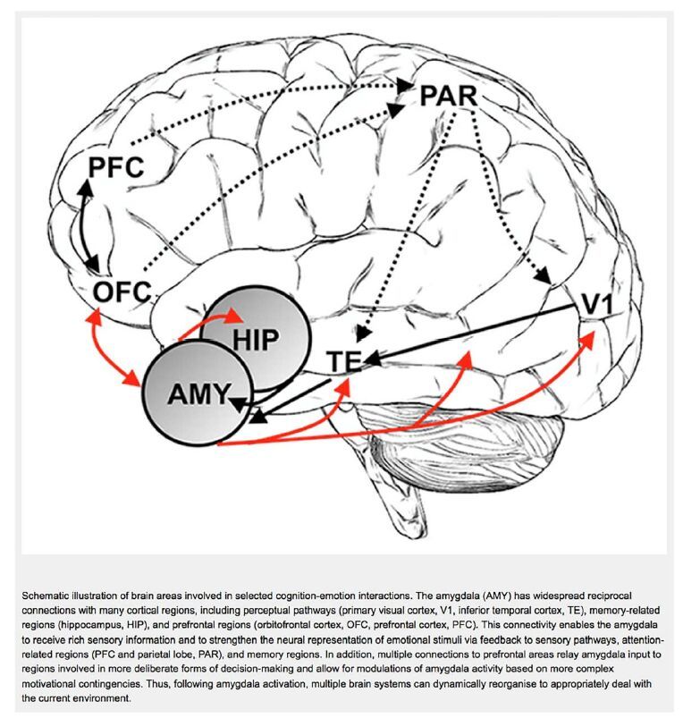
[17] | Floresco SB, Ghods-Sharifi S (2006) Amygdala-Prefrontal Cortical Circuitry Regulates Effort-Based Decision Making. https://cercor.oxfordjournals.org/content/17/2/251.full |
[18] | Collins F (2012) “The Symphony Inside Your Brain” Posted on November 5, 2012http://directorsblog.nih.gov/2012/11/05/the-symphony-inside-your-brain/ |
[19] | Seifter J, Economy P (2001) Leadership Ensemble. New York, NY: Henry Holt & Co. |
[20] | Seifter J, Economy P (2001) Leader to Leader, No. 1, Summer. |
[21] | De Dreu CK, Baas M, Roskes M, et al. (2014) Oxytonergic circuitry sustains and enables creative cognition in humans. Soc Cogn Affect Neurosci 9: 1159-1165. doi: 10.1093/scan/nst094 |
[22] |
Siler T (2012) Neuro-impressions: interpreting the nature of human creativity. Front Hum Neurosci 6: 1-5. doi: 10.3389/fnhum.2012.00282 doi: 10.3389/fnhum.2012.00282
![]() |
[23] | Polanyi M (1958/1998) Personal Knowledge. Towards a Post Critical Philosophy. London: Routledge. |
[24] | Polanyi M (1967) The Tacit Dimension. New York, NY: Anchor Books. |
[25] | Siler T (1986) Architectonics of Thought: A Symbolic Model of Interdisciplinary Studies in Psychology and Art, Massachusetts Institute of Technology. Available at: https://dspace.mit.edu/handle/1721.1/17200 |
[26] | Siler T (1993) Cerebralism: Creating A New Millennium of Minds, Bodies and Civilizations. New York, NY: Ronald Feldman Fine Arts. |
[27] | Siler T (1981) Reality. Master’s Thesis, Master of Science in Visual Studies, Center for Advanced Visual Studies, Massachusetts Institute of Technology. |
[28] | Siler T (1983) The Biomirror. New York, NY: Ronald Feldman Fine Arts. |
[29] | Schacter DL (1996) Searching for Memory: The Brain, the Mind and the Past. New York, NY: Basic Books. |
[30] | Ramachandran VS, Hirstein W (1999) The science of art. J Conscious Studies 6: 15-51. |
[31] | Ramachandran VS (2011) The Tell-Tale Brain. New York, NY: Norton. |
[32] | Siler T (2015) Neuroart: picturing the neuroscience of intentional actions in art and science. http://journal.frontiersin.org/article/10.3389/fnhum.2015.00410/abstract |
[33] | Kandel ER (2012) The Age of Insight: The quest to understand the unconscious in art, mind, brain, from Vienna 1900 to the Present. New York, NY: Random House. |
[34] | Siler T (1990) Breaking The Mind Barrier. New York, NY: Simon and Schuster, p.254. |
[35] | Siler T (1987) The Art of Thought. Centre Saidye Bronfman, Montreal, Canada; and Ronald Feldman Fine Arts, New York, NY. |
[36] | Bem JB (2011) “Feeling the Future: Experimental Evidence for Anomalous Retroactive Influences on Cognition and Affect.” J Personality Soc Psychology 100: 407-425. http://dx.doi.org/10.1037/a0021524 |
[37] | Siler T (1986) Architectonics of Thought: A Symbolic Model of Interdisciplinary Studies in Psychology and Art, Massachusetts Institute of Technology. Available at: https://dspace.mit.edu/handle/1721.1/17200 |
[38] | Morrison P, Tsipis K (1998) Reason Enough To Hope: America and the World of the 21st Century. Cambridge, MA: The MIT Press (p. 198). |
[39] | Bishop SJ (2007) Neurocognitive mechanisms of anxiety: an integrative account. Trend Cognitive Sci. doi:10.1016/j.tics.2007.05.008 |
[40] | Floresco SB, Ghods-Sharifi S (2006) Amygdala-Prefrontal Cortical Circuitry Regulates Effort-Based Decision Making. https://cercor.oxfordjournals.org/content/17/2/251.full |
[41] | Aggleton JP (Ed.) (1992) The amygdala: neurobiological aspects of emotions, memory and mental dysfunction. New York: Wiley-Liss Inc. |
[42] |
Saddoris MP, Gallagher M, Schoenbaum G (2005) Rapid associative encoding in basolateral amygdala depends on connections with orbitofrontal cortex. Neuron 46:321-331. doi: 10.1016/j.neuron.2005.02.018
![]() |
[43] | Bishop SJ (2007) Neurocognitive mechanisms of anxiety: an integrative account. Trend Cognitive Sci. doi:10.1016/j.tics.2007.05.008 |
[44] | Eliasmith C, Stewart TC, Xuan Choo, et al. (2012) A Large-Scale Model of the Functioning Brain. Science 338: 1202-1205. DOI: 10.1126/science.1225266 |
[45] | Morrison JG, Kelly RT, Moore RA, et al. (2003) Tactical Decision Making Under Stress (TADMUS) Decision Support System unclassified paper sponsored by the Office of Naval Research, Cognitive and Neural Science Technology Division. |
[46] | Bishop SJ (2007) Neurocognitive mechanisms of anxiety: an integrative account. Trend Cognitive Sci. doi:10.1016/j.tics.2007.05.008 |
[47] | Jackson PL, Brunet E, Meltzoff AN, et al. (2006) Empathy examined through the neural mechanisms involved in imagining how I feel versus how you feel pain. Neuropsychologia 44: 752-761. |
[48] | Freedberg D, Gallese V (2014) Motion, emotion and empathy in esthetic experience. Trend Cognitive Sci 11: 197-203. |
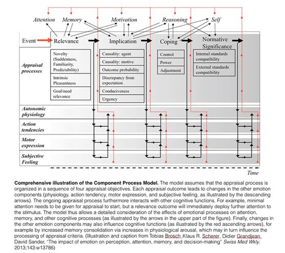
[49] | Brosch T, Scherer KR, Grandjean D, Sander D. (2013) The impact of emotion on perception, attention, memory, and decision-making. Medical Intelligence. Swiss Med Wkly. 2013 May 14; 143: w13786. doi: 10.4414/smw.2013.13786. |
[50] | Phelps EA (2004) Human emotion and memory: interactions of the amygdala and hippocampal complex. Current Opinion Neurobiology 14: 198-202. DOI 10.1016/j.conb.2004.03.015 |
[51] |
Gross JJ (1998) The Emerging Field of Emotion Regulation: An Integrative Review. Rev General Psychology 2: 271-299. doi: 10.1037/1089-2680.2.3.271
![]() |
[52] | Hou X, Zhang L (2008) “Dynamic visual attention: searching for coding length increments. Advances Neural Information Processing Systems 21 (NIPS 2008)Neural Information Processing Systems (NIPS) |
[53] |
Chen Q, Weidner R, Vossel S, et al. (2012) Neural Mechanisms of Attentional Reorienting in Three-Dimensional Space. J Neurosci 32: 13352-13362. doi: 10.1523/JNEUROSCI.1772-12.2012
![]() |
[54] | Greicius MD, Srivastava G, Reiss AL, et al. (2004) Default-mode network activity distinguishes Alzheimer’s disease from healthy aging: evidence from functional MRI. Proc Natl Acad Sci U.S.A. 101: 4637-4642. |
[55] | Andreasen NC, O’Leary DS, Cizadlo T, et al. (1995) Remembering the past: two facets of episodic memory explored with positron emission tomography. Am J Psychiatry 152: 1576-1585. |
[56] | Buckner RL, Andrews-Hanna JR, Schacter DL (2008) The Brain’s Default Network Anatomy, Function, and Relevance to Disease. Ann NY Acad Sci 1124: 1-38. New York Academy of Sciences. doi: 10.1196/annals.1440.011 |
[57] | Arrien J (2015) http://www.nsf.gov/mobile/discoveries/disc_images.jspcntn_id=136954&org=NSF |
[58] | Contreras-Vidal J, Prasad S, Roysam B (2015) NCS-FO: Assaying neural individuality and variation in freely behaving people based on qEEG. NSF-Award Abstract #1533691 |
[59] | Bruya B (2010) Effortless Attention: A New Perspective in the Cognitive Science of Attention and Action. Cambridge, MA: Bradford Books. |
[60] | Siler T (2015) Neuroart: picturing the neuroscience of intentional actions in art and science. http://journal.frontiersin.org/article/10.3389/fnhum.2015.00410/abstract |
[61] |
Cohen D (1972) Magnetoencephalography: detection of the brain's electrical activity with a superconducting magnetometer. Science 175: 664-666. doi: 10.1126/science.175.4022.664
![]() |
[62] | Encyclopedia of the Neurological Sciences (p. 293). |
[63] | Kreiman G, Rutishauser U, Cerf M, et al. (2014) The next ten years and beyond. In single neuron studies of the human brain. In Probing Cognition, eds I. Fried U, Rutishauser M, Cerf G Kreiman (Cambridge, MA: The MIT Press), 347-358. |
[64] | Floresco SB, Ghods-Sharifi S (2006) Amygdala-Prefrontal Cortical Circuitry Regulates Effort-Based Decision Making. https://cercor.oxfordjournals.org/content/17/2/251.full |
[65] | Hickok G, Poeppel D (2000) Towards a functional neuroanatomy of speech perception. Trend Cognitive Sci 4: 131-138. DOI: 10.1016/S1364-6613(00)01463-7 |
[66] | Hickok G, Poeppel D (2004) Dorsal and ventral streams: a framework for understanding aspects of the functional anatomy of language. Cognition 92: 67-99 DOI: 10.1016/j.cognition.2003.10.011 |
[67] | Hickok G, Poeppel D (2007) The cortical organization of speech processing. Nat Rev Neurosci 8: 393-402. DOI: 10.1038/nrn2113 |
[68] | Lehrer J (2011) The Science of Irrationality. A Nobelist explains our fondness for not thinking. The Wall Street J. October 15-16; C18. |
[69] | Siler T (2015) Neuroart: picturing the neuroscience of intentional actions in art and science. http://journal.frontiersin.org/article/10.3389/fnhum.2015.00410/abstract |
[70] | Siler T (1997) Think Like A Genius: Use Your Creativity in Ways That Will Enrich Your Life. New York: Bantam Books. |
[71] | Siler T (2011) The ArtScience Program for Realizing Human Potential. Leonardo 44, 417-424. doi: 10.1162/leon_a_00242 |
[72] |
Root-Bernstein B, Siler T, Brown A, et al. (2011) ArtScience: integrative collaboration to create a sustainable future. Leonardo 44: 192. doi: 10.1162/leon_e_00161 doi: 10.1162/LEON_e_00161
![]() |
[73] | Adolphs R (2015) The unsolved problems of neuroscience. Trend Cognitive Sci. PMID: 25703689 |
[74] |
Adee S (2008) Reverse engineering the brain. IEEE Spectrum 45: 51-55. doi: 10.1109/MSPEC.2008.4531462
![]() |
1. | An Ma, Qimin Zhang, Global attractor and threshold dynamics of a reaction–diffusion population model in a polluted environment, 2023, 69, 1598-5865, 989, 10.1007/s12190-022-01781-4 | |
2. | An Ma, Shuting Lyu, Qimin Zhang, Stationary distribution and optimal control of a stochastic population model in a polluted environment, 2022, 19, 1551-0018, 11260, 10.3934/mbe.2022525 | |
3. | An Ma, Jing Hu, Qimin Zhang, DYNAMIC ANALYSIS AND OPTIMAL CONTROL OF A TOXICANT-POPULATION MODEL WITH REACTION-DIFFUSION, 2024, 14, 2156-907X, 579, 10.11948/20210438 | |
4. | An Ma, Jing Hu, Ming Ye, Qimin Zhang, Investigation of sliding mode dynamics and near-optimal controls for a reaction–diffusion population model in a polluted environment, 2024, 79, 09473580, 101097, 10.1016/j.ejcon.2024.101097 |