Sleep is a complex physiological process that is regulated globally, regionally, and locally by both cellular and molecular mechanisms. It occurs to some extent in all animals, although sleep expression in lower animals may be co-extensive with rest. Sleep regulation plays an intrinsic part in many behavioral and physiological functions. Currently, all researchers agree there is no single physiological role sleep serves. Nevertheless, it is quite evident that sleep is essential for many vital functions including development, energy conservation, brain waste clearance, modulation of immune responses, cognition, performance, vigilance, disease, and psychological state. This review details the physiological processes involved in sleep regulation and the possible functions that sleep may serve. This description of the brain circuitry, cell types, and molecules involved in sleep regulation is intended to further the reader’s understanding of the functions of sleep.
Citation: Mark R. Zielinski, James T. McKenna, Robert W. McCarley. Functions and Mechanisms of Sleep[J]. AIMS Neuroscience, 2016, 3(1): 67-104. doi: 10.3934/Neuroscience.2016.1.67
Sleep is a complex physiological process that is regulated globally, regionally, and locally by both cellular and molecular mechanisms. It occurs to some extent in all animals, although sleep expression in lower animals may be co-extensive with rest. Sleep regulation plays an intrinsic part in many behavioral and physiological functions. Currently, all researchers agree there is no single physiological role sleep serves. Nevertheless, it is quite evident that sleep is essential for many vital functions including development, energy conservation, brain waste clearance, modulation of immune responses, cognition, performance, vigilance, disease, and psychological state. This review details the physiological processes involved in sleep regulation and the possible functions that sleep may serve. This description of the brain circuitry, cell types, and molecules involved in sleep regulation is intended to further the reader’s understanding of the functions of sleep.

| [1] |
Siegel JM (2008) Do all animals sleep? Trends Neurosci 31: 208-213. doi: 10.1016/j.tins.2008.02.001

|
| [2] |
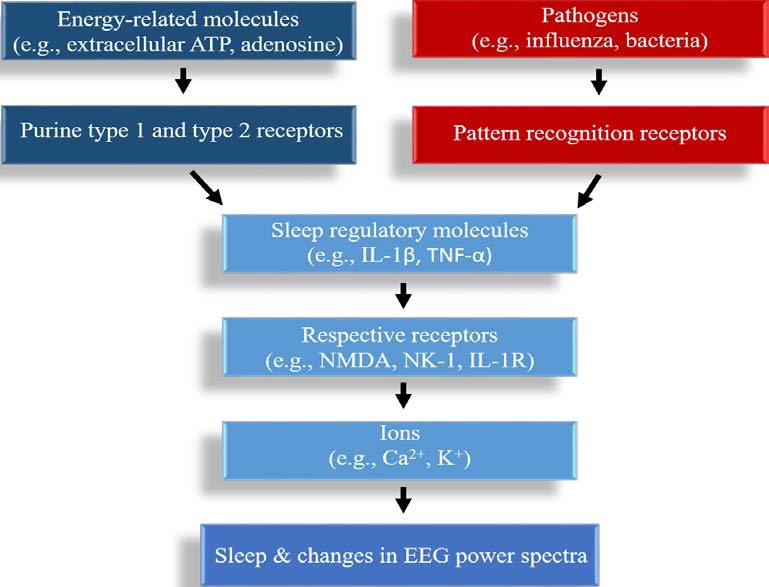
Zielinski MR, Krueger JM (2011) Sleep and innate immunity. Front Biosci (Schol Ed) 3: 632-642. doi: 10.2741/s176
|
| [3] |
Etinger U, Kumari V (2015) Effects of sleep deprivation on inhibitory biomarkers of schizophrenia: implications of drug development. Lancet Psychiatry 2: 1028-1035. doi: 10.1016/S2215-0366(15)00313-2
|
| [4] |
Allada R, Siegel JM (2008) Unearthing the phylogenetic roots of sleep. Curr Biol 18: R670-R679. doi: 10.1016/j.cub.2008.06.033
|
| [5] | Kishi A, Yasuda H, Matsumoto T, et al. (2011) NREM sleep stage transitions control ultradian REM sleep rhythm. Sleep 34:1423-1432. |
| [6] |
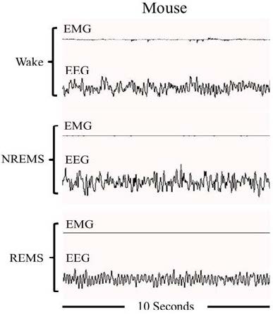
Dement W, Kleitman N (1957) The relation of eye movements during sleep to dream activity: an objective method for the study of dreaming. J Experiment Psychol 53: 339-346. doi: 10.1037/h0048189
|
| [7] | Schomer DL, da Silva FL (2010) Niedermeyer's Electroencephalography: Basic Principles, Clinical Applications, and Related Fields. Lippincott Williams & Wilkins, Philadelphia, PA. |
| [8] | Canton R (1877) Interim report on investigations of the electric currents of the brain. British Med J 1: 62-65. |
| [9] | Danilewsky WY (1877) Investigations into the physiology of the brain. Doctoral thesis, University of Charkov. |
| [10] | Yeo GF (1881) Transactions of the 7th International Medical Congress. Volume 1. Edited by W. MacCormac London: J.W. Kolkmann. |
| [11] | Ferrier D (1881) Transactions of the 7th International Medical Congress. Volume 1. Edited by W. MacCormac London: J.W. Kolkmann. |
| [12] | Beck A (1891) Oznaczenie lokalzacji w mózgu I rdzeniu za pomoc zjawisk elektycznych. Rozprawy Akademii Umietjtnoci, Wydzia Matematyczno. 1: 187-232. |
| [13] | Pravdich-Neminsky V (1913) Ein Versuch der Registrierung der elektrischen Gehirnerscheinungen. Zentralblatt fur Physiologie 27: 951-960. |
| [14] |
Berger H (1929) über das Elektronkephalogramm. Arch Psychiat Nervenkrank 87: 527-570. doi: 10.1007/BF01797193
|
| [15] |
Aserinsky E, Kleitman N (1953) Regularly occurring periods of eye motility, and concomitant phenomena, during sleep. Science 118: 273-274. doi: 10.1126/science.118.3062.273
|
| [16] |
Dement W (1958) The occurrence of low voltage, fast electroencephalogram patterns during behavioral sleep in the cat. Electroencephalogr Clin Neurophysiol 10: 291-296. doi: 10.1016/0013-4694(58)90037-3
|
| [17] | Jouvet M, Michel F, Courjon J (1959) Sur une stade d’activité électrique cérébrale rapide au cours du sommeil physiologique. C R Soc Biol 153: 1024-1028. |
| [18] | Fields RD (2008) Oligodendrocytes changing the rules: action potentials in glia and oligodendrocytes controlling action potentials; Neuroscientist 14: 540-543. |
| [19] |
Fields RD (2010) Release of neurotransmitters from glia. Neuron Glia Biol 6: 137-139. doi: 10.1017/S1740925X11000020
|
| [20] | Buzsáki G, Logothetis N, Singer W (2013) Scaling Brain Size, Keeping Timing: Evolutionary Preservation of Brain Rhythms. Neuron 80: 751-764. |
| [21] |
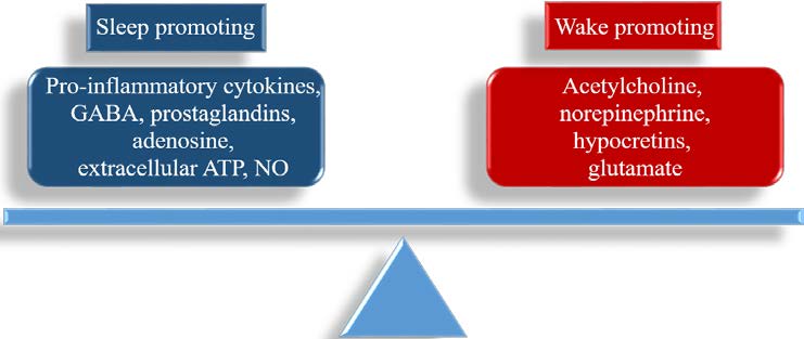
Brown RE, Basheer R, McKenna JT, et al. (2012) Control of sleep and wakefulness. Physiol Rev 92: 1087-1187. doi: 10.1152/physrev.00032.2011
|
| [22] |
Zielinski MR, Gerashchenko L, Karpova SA, et al. (2013) A novel telemetric system to measure polysomnographic biopotentials in freely moving animals. J Neurosci Methods 216: 79-86. doi: 10.1016/j.jneumeth.2013.03.022
|
| [23] | Steriade M, Conteras D, Curro, et al. (1993) The slow (< 1 Hz) oscillation in reticular thalamic and thalamocortical neurons: scenario of sleep rhythm generation in interacting thalamic and neocortical networks. J Neurosci 13: 3284-3299. |
| [24] | Steriade M, Timofeev I, Grenier F (2001) Natural waking and sleep states: a view from inside neocortical neurons. J Neurophysiol 85: 1969-1985. |
| [25] |
Dang-Vu TT, Schabus M, Desseilles M, et al. (2008) Spontaneous neural activity during human slow wave sleep. Proc Natl Acad Sci U.S.A. 105: 15160-15165. doi: 10.1073/pnas.0801819105
|
| [26] | Achermann P (2004) The two-process model of sleep regulation revisited. Aviat Space Environ Med 75: A37-43. |
| [27] |
Sollars APJ, Pickard GE (2015) The neurobiology of circadian rhythms. Psychiatr Clin North Am 38: 645-665. doi: 10.1016/j.psc.2015.07.003
|
| [28] | Dijk DJ, Czeisler CA (1995) Contribution of the circadian pacemaker and the sleep homeostat to sleep propensity, sleep structure, electroencephalographic slow waves, and sleep spindle activity in humans. J Neurosci 15: 3526-3538. |
| [29] | Davis CJ, Clinton JM, Jewett KA, et al. (2011) Delta wave power: an independent sleep phenotype or epiphenomenon? J Clin Sleep Med 7: S16-18. |
| [30] |
Steriade M (2006) Grouping of brain rhythms in corticothalamic systems. Neuroscience 137: 1087-1106. doi: 10.1016/j.neuroscience.2005.10.029
|
| [31] | Gerashchenko D, Matsumura H (1996) Continuous recordings of brain regional circulation during sleep/wake state transitions in rats. Am J Physiol 270: R855-863. |
| [32] | Phillips DJ, Schei JL, Rector DM (2013) Vascular compliance limits during sleep deprivation and recovery sleep. Sleep 36: 1459-1470. |
| [33] |
Ngo HV, Martinetz T, Born J, et al. (2013) Auditory closed-loop stimulation of the sleep slow oscillation enhances memory. Neuron 78: 545-553. doi: 10.1016/j.neuron.2013.03.006
|
| [34] |
Marshall L, Kirov R, Brade J, et al. (2011) Transcranial electrical currents to probe EEG brain rhythms and memory consolidation during sleep in humans. PLoS One 6: e16905. doi: 10.1371/journal.pone.0016905
|
| [35] |
Pace-Schott EF, Spencer RM (2011) Age-related changes in the cognitive function of sleep. Prog Brain Res 191: 75-89. doi: 10.1016/B978-0-444-53752-2.00012-6
|
| [36] |
Lisman J (2012) Excitation, inhibition, local oscillations, or large-scale loops: what causes the symptoms of schizophrenia? Curr Opin Neurobiol 22: 537-544. doi: 10.1016/j.conb.2011.10.018
|
| [37] |
Pignatelli M, Beyeler A, Leinekugel X (2012) Neural circuits underlying the generation of theta oscillations. J Physiol Paris 106: 81-92. doi: 10.1016/j.jphysparis.2011.09.007
|
| [38] |
Lu J, Sherman D, Devor M, et al. (2006) A putative flip-flop switch for control of REM sleep. Nature 441: 589-594. doi: 10.1038/nature04767
|
| [39] |
Abel T, Havekes R, Saletin JM et al. (2013) Sleep, plasticity and memory from molecules to whole-brain networks. Curr Biol 23: R774-788. doi: 10.1016/j.cub.2013.07.025
|
| [40] |
Bhattacharya BS, Coyle D, Maguire LP (2011) Alpha and theta rhythm abnormality in Alzheimer’s Disease: a study using a computational model. Adv Exp Med Biol 718: 57-73. doi: 10.1007/978-1-4614-0164-3_6
|
| [41] | Bian Z, Li Q, Wang L, et al. (2014) Relative power and coherence of EEG series are related to amnestic mild cognitive impairment in diabetes. Front Aging Neurosci 6: 11. |
| [42] |
Iranzo A, Isetta V, Molinuevo JL, et al. (2010) Electroencephalographic slowing heralds mild cognitive impairment in idiopathic REM sleep behavior disorder. Sleep Med 11: 534-539. doi: 10.1016/j.sleep.2010.03.006
|
| [43] |
Ba?ar E (2012) A review of alpha activity in integrative brain function: fundamental physiology, sensory coding, cognition and pathology. Int J Psychophysiol 86: 1-24. doi: 10.1016/j.ijpsycho.2012.07.002
|
| [44] | Jaimchariyatam N, Rodriguez CL, Budur K (2011) Prevalence and correlates of alpha-delta sleep in major depressive disorders. Innov Clin Neurosci 8: 35-49. |
| [45] |
Engel AK, Fries P (2010) Beta-band oscillations--signaling the status quo? Curr Opin Neurobiol 20: 156-165. doi: 10.1016/j.conb.2010.02.015
|
| [46] |
Buzsáki G, Wang XJ (2012) Mechanisms of gamma oscillations. Annu Rev Neurosci 35: 203-225. doi: 10.1146/annurev-neuro-062111-150444
|
| [47] |
Cardin JA, Carlén M, Meletis K, et al. (2009) Driving fast-spiking cells induces gamma rhythm and controls sensory responses. Nature 459: 663-667. doi: 10.1038/nature08002
|
| [48] |
Sohal VS, Zhang F, Yizhar O, et al. (2009) Parvalbumin neurons and gamma rhythms enhance cortical circuit performance. Nature 459: 698-702. doi: 10.1038/nature07991
|
| [49] | Yang C, McKenna JT, Zant JC, et al. (2014) Cholinergic neurons excite cortically projecting basal forebrain GABAergic neurons. J Neurosci 692: 79-85. |
| [50] |
Kim T, Thankachan S, McKenna JT,et al. (2015) Cortically projecting basal forebrain parvalbumin neurons regulate cortical gamma band oscillations. Proc Natl Acad Sci U.S.A. 112: 3535-3540. doi: 10.1073/pnas.1413625112
|
| [51] | Frank MG, Heller HC (2003) The ontogeny of mammalian sleep: a reappraisal of alternative hypotheses. J Sleep Res 12: 25-34. |
| [52] | Mirmiran M, Scholtens J, van de Poll NE, et al. (1983) Effects of experimental suppression of active (REM) sleep during early development upon adult brain and behavior in the rat. Brain Res 283: 277-286. |
| [53] |
Rasch B, Born J (2013) About sleep's role in memory. Physiol Rev 93: 681-766. doi: 10.1152/physrev.00032.2012
|
| [54] | Zielinski MR, Gerashchenko D (2015) Role of sleep in cognition, immunity, and disease and its interaction with exercise. Diet and Exercise in cognitive function and neurological diseases. Farooqui T, Farooqui AA. pp 225-240. |
| [55] |
Tononi G, Cirelli C (2014) Sleep and the price of plasticity: from synaptic and cellular homeostasis to memory consolidation and integration. Neuron 81: 12-34. doi: 10.1016/j.neuron.2013.12.025
|
| [56] | Frank MG (2012) Erasing synapses in sleep: is it time to be SHY? Neural Plasticity 264378. |
| [57] |
Von Economo C (1930) Sleep as a problem of localization. The Journal of Nervous and Mental Disease 71: 249–259. doi: 10.1097/00005053-193003000-00001
|
| [58] |
Bargmann CI, Marder E (2013) From the connectome to brain function. Nat Methods 10: 483-490. doi: 10.1038/nmeth.2451
|
| [59] |
Moruzzi G, Magoun HW (1949) Brain stem reticular formation and activation of the EEG. Electroencephalogr Clin Neurophysiol 1: 455-473. doi: 10.1016/0013-4694(49)90219-9
|
| [60] |
Fuller PM, Gooley JJ, Saper CB (2006) Neurobiology of the sleep-wake cycle: sleep architecture, circadian regulation, and regulatory feedback. J Biol Rhythms 21: 482-493. doi: 10.1177/0748730406294627
|
| [61] |
Saper CB, Scammell TE, Lu J (2005) Hypothalamic regulation of sleep and circadian rhythms. Nature 437: 1257-1263. doi: 10.1038/nature04284
|
| [62] |
Saper CB, Chou TC, Scammell TE (2001) The sleep switch: hypothalamic control of sleep and wakefulness. Trends Neurosci 24: 726-731. doi: 10.1016/S0166-2236(00)02002-6
|
| [63] |
Li S, Varga V, Sik A, et al. (2005) GABAergic control of the ascending input from the median raphe nucleus to the limbic system. J Neurophysiol 94: 2561-2574. doi: 10.1152/jn.00379.2005
|
| [64] |
Takahashi K, Lin JS, Sakai K (2006) Neuronal activity of histaminergic tuberomammillary neurons during wake-sleep states in the mouse. J Neurosci 26: 10292-10298. doi: 10.1523/JNEUROSCI.2341-06.2006
|
| [65] |
Saper CB, Fuller PM, Pedersen NP, et al. (2010) Sleep state switching. Neuron. 68: 1023-1042. doi: 10.1016/j.neuron.2010.11.032
|
| [66] |
Hur EE, Zaborszky L (2005) Vglut2 afferents to the medial prefrontal and primary somatosensory cortices: a combined retrograde tracing in situ hybridization study. J Comp Neurol 483: 351-373. doi: 10.1002/cne.20444
|
| [67] |
Saper CB, Loewy AD (1980) Efferent connections of the parabrachial nucleus in the rat. Brain Res 197: 291-317. doi: 10.1016/0006-8993(80)91117-8
|
| [68] |
Levey AI, Hallanger AE, Wainer BH (1987) Cholinergic nucleus basalis neurons may influence the cortex via the thalamus. Neurosci Lett 74: 7-13. doi: 10.1016/0304-3940(87)90042-5
|
| [69] |
Asanuma C, Porter LL (1990) Light and electron microscopic evidence for a GABAergic projection from the caudal basal forebrain to the thalamic reticular nucleus in rats. J Comp Neurol 302: 159-172. doi: 10.1002/cne.903020112
|
| [70] | Manning KA, Wilson JR, Uhlrich DJ (1996) Histamine-immunoreactive neurons and their innervation of visual regions in the cortex, tectum, and thalamus in the primate Macaca mulatta. J Comp Neurol 373: 271-282. |
| [71] | Zikopoulos B, Barbas H (2007) Circuits form multisensory integration and attentional modulation through the prefrontal cortex and the thalamic reticular nucleus in primates. Rev Neurosci 18: 417-438. |
| [72] |
Asanuma C (1992) Noradrenergic innervation of the thalamic reticular nucleus: a light and electron microscopic immunohistochemical study in rats. J Comp Neurol 319: 299-311. doi: 10.1002/cne.903190209
|
| [73] |
Jones BE (2004) Activity, modulation and role of basal forebrain cholinergic neurons innervating the cerebral cortex. Prog Brain Res 145: 157-169. doi: 10.1016/S0079-6123(03)45011-5
|
| [74] |
Xu M, Chung S, Zhang S, et al. (2015) Basal forebrain circuit for sleep-wake control. Nat Neurosci 18: 1641-1647. doi: 10.1038/nn.4143
|
| [75] |
Freund TF, Meskenaite V (1992) Gamma-Aminobutyric acid-containing basal forebrain neurons innervate inhibitory interneurons in the neocortex. Proc Natl Acad Sci U.S.A. 89: 738-742. doi: 10.1073/pnas.89.2.738
|
| [76] |
Henny P, Jones BE (2008) Projections from basal forebrain to prefrontal cortex comprise cholinergic, GABAergic and glutamatergic inputs to pyramidal cells or interneurons. Eur J Neurosci 27: 654-670. doi: 10.1111/j.1460-9568.2008.06029.x
|
| [77] |
McGinty DJ, Sterman MB (1968) Sleep suppression after basal forebrain lesions in the cat. Science 160: 1253-1255. doi: 10.1126/science.160.3833.1253
|
| [78] |
Sherin JE, Shiromani PJ, McCarley RW, et al. (1996) Activation of ventrolateral preoptic neurons during sleep. Science 271: 216-219. doi: 10.1126/science.271.5246.216
|
| [79] |
Szymusiak R, McGinty D (1986) Sleep-related neuronal discharge in the basal forebrain of cats. Brain Res 370: 82-92. doi: 10.1016/0006-8993(86)91107-8
|
| [80] |
Suntsova NV, Dergacheva OY (2004) The role of the medial preoptic area of the hypothalamus in organizing the paradoxical phase of sleep. Neurosci Behav Physiol 34: 29-35. doi: 10.1023/B:NEAB.0000003243.95706.de
|
| [81] |
Alam MA, Kumar S, McGinty D, et al. (2014) Neuronal activity in the preoptic hypothalamus during sleep deprivation and recovery sleep. J Neurophysiol 111: 287-99. doi: 10.1152/jn.00504.2013
|
| [82] |
Hassani OK, Lee MG, Jones BE (2009) Melanin-concentrating hormone neurons discharge in a reciprocal manner to orexin neurons across the sleep-wake cycle. Proc Natl Acad Sci U.S.A. 106: 2418-2422. doi: 10.1073/pnas.0811400106
|
| [83] |
Verret L, Goutagny R, Fort P et al. (2003) A role of melanin-concentrating hormone producing neurons in the central regulation of paradoxical sleep. BMC Neurosci 4: 19. doi: 10.1186/1471-2202-4-19
|
| [84] |
Jego S, Glasgow SD, Herrera CG et al. (2013) Optogenetic identification of a rapid eye movement sleep modulatory circuit in the hypothalamus. Nat Neurosci 16: 1637-1643. doi: 10.1038/nn.3522
|
| [85] | Jouvet M (1962) Research on the neural structures and responsible mechanisms in different phases of physiological sleep. Arch Ital Biol 100: 125-206. |
| [86] |
Hobson JA, McCarley RW, Wyzinski PW (1975) Sleep cycle oscillation: reciprocal discharge by two brainstem neuronal groups. Science 189: 55-58. doi: 10.1126/science.1094539
|
| [87] | McCarley RW, Massaquoi SG (1986) Further discussion of a model of the REM sleep oscillator. Am J Physiol 251: R1033-1036. |
| [88] |
Boissard R, Gervasoni D, Schmidt MH, et al. (2002) The rat ponto-medullary network responsible for paradoxical sleep onset and maintenance: a combined microinjection and functional neuroanatomical study. Eur J Neurosci 16: 1959-1973. doi: 10.1046/j.1460-9568.2002.02257.x
|
| [89] | Sakai K, Jouvet M (1980) Brain stem PGO-on cells projecting directly to the cat dorsal lateral geniculate nucleus. Brain Res 194: 500-505. |
| [90] |
Peigneux P, Laureys S, Fuchs S et al. (2001) Generation of rapid eye movements during paradoxical sleep in humans. Neuroimage 14: 701-708. doi: 10.1006/nimg.2001.0874
|
| [91] | Lim AS, Lozano AM, Moro E, et al. (2007) Characterization of REM-sleep associated ponto-geniculo-occipital waves in the human pons. Sleep 30: 823-827. |
| [92] | Datta S, Siwek DF, Patterson EH, et al. (1998) Localization of pontine PGO wave generation sites and their anatomical projections in the rat. Synapse 30: 409-423. |
| [93] |
El Mansari M, Sakai K, Jouvet M (1989) Unitary characteristics of presumptive cholinergic tegmental neurons during the sleep-waking cycle in freely moving cats. Exp Brain Res 76: 519-529. doi: 10.1007/BF00248908
|
| [94] | Fahrenkrug J, Emson PC (1997) Vasoactive intestinal polypeptide: functional aspects. Br Med Bull 38: 265-270. |
| [95] |
Takahashi K, Kayama Y, Lin JS, et al. (2010) Locus coeruleus neuronal activity during the sleep-waking cycle in mice. Neuroscience 169: 1115-1126. doi: 10.1016/j.neuroscience.2010.06.009
|
| [96] |
Steininger TL, Alam MN, Gong H, et al. (1999) Sleep-waking discharge of neurons in the posterior lateral hypothalamus of the albino rat. Brain Res 840: 138-147. doi: 10.1016/S0006-8993(99)01648-0
|
| [97] |
Trulson ME, Jacobs BL, Morrison AR (1981) Raphe unit activity during REM sleep in normal cats and in pontine lesioned cats displaying REM sleep without atonia. Brain Res 226: 75-91. doi: 10.1016/0006-8993(81)91084-2
|
| [98] |
Waszkielewicz AM, Gunia A, Szkaradek N, et al. (2013) Ion channels as drug targets in central nervous system disorders. Curr Med Chem 20: 1241-1285. doi: 10.2174/0929867311320100005
|
| [99] |
Kirschstein T, K?hling R (2009) What is the source of the EEG? Clin EEG Neurosci 40: 146-149. doi: 10.1177/155005940904000305
|
| [100] |
Born J, Feld GB (2012) Sleep to upscale, sleep to downscale: balancing homeostasis and plasticity. Neuron 75: 933-935. doi: 10.1016/j.neuron.2012.09.007
|
| [101] |
Littleton JT, Ganetzky B (2000) Ion channels and synaptic organization: analysis of the Drosophila genome. Neuron 26: 35-43. doi: 10.1016/S0896-6273(00)81135-6
|
| [102] |
Cirelli C, Bushey D, Hill S, et al. (2005) Reduced sleep in Drosophila Shaker mutants. Nature 434: 1087-1092. doi: 10.1038/nature03486
|
| [103] |
Koh K, Joiner WJ, Wu MN, et al. (2008) Identification of SLEEPLESS, a sleep-promoting factor. Science 321: 372-376. doi: 10.1126/science.1155942
|
| [104] |
Bushey D, Huber R, Tononi G, et al. (2007) Drosophila Hyperkinetic mutants have reduced sleep and impaired memory. J Neurosci 27: 5384-5393. doi: 10.1523/JNEUROSCI.0108-07.2007
|
| [105] |
Douglas CL, Vyazovskiy V, Southard T, et al. (2007) Sleep in Kcna2 knockout mice. BMC Biol 5: 42. doi: 10.1186/1741-7007-5-42
|
| [106] |
Espinosa F, Marks G, Heintz N, et al. (2004) Increased motor drive and sleep loss in mice lacking Kv3-type potassium channels. Genes Brain Behav 3: 90-100. doi: 10.1046/j.1601-183x.2003.00054.x
|
| [107] | Joho RH, Ho CS, Marks GA (1999) Increased gamma- and decreased delta-oscillations in a mouse deficient for a potassium channel expressed in fast-spiking interneurons. J Neurophysiol 82: 1855-1864. |
| [108] |
Cui SY, Cui XY, Zhang J, et al. (2011) Ca2+ modulation in dorsal raphe plays an important role in NREM and REM sleep regulation during pentobarbital hypnosis. Brain Res 1403: 12-18. doi: 10.1016/j.brainres.2011.05.064
|
| [109] |
Crunelli V, Cope DW, Hughes SW (2006) Thalamic T-type Ca2+ channels and NREM sleep. Cell Calcium 40: 175-190. doi: 10.1016/j.ceca.2006.04.022
|
| [110] | Anderson MP, Mochizuki T, Xie J, et al. (2005) Thalamic Cav3.1 T-type Ca2+ channel plays a crucial role in stabilizing sleep. Proc Natl Acad Sci USA 102: 1743-1748. |
| [111] |
Lee J, Kim D, Shin HS (2004) Lack of delta waves and sleep disturbances during non-rapid eye movement sleep in mice lacking alpha1G-subunit of T-type calcium channels. Proc Natl Acad Sci USA 101: 18195-18199. doi: 10.1073/pnas.0408089101
|
| [112] |
David F, Schmiedt JT, Taylor HL, et al. (2013) Essential thalamic contribution to slow waves of natural sleep. J Neurosci 33: 19599-19610. doi: 10.1523/JNEUROSCI.3169-13.2013
|
| [113] | Hortsch M (2009) A short history of the synapse-Golgi versus Ramon y Cajal. The Sticky Synapse: 1-9. |
| [114] |
de Lecea L, Kilduff TS, Peyron C, et al. (1998) The hypocretins: hypothalamus-specific peptides with neuroexcitatory activity. Proc Natl Acad Sci USA 95: 322-327. doi: 10.1073/pnas.95.1.322
|
| [115] |
Sakurai T, Amemiya A, Ishii M, et al. (1998) Orexins and orexin receptors: a family of hypothalamic neuropeptides and G protein-coupled receptors that regulate feeding behavior. Cell 92: 573-585. doi: 10.1016/S0092-8674(00)80949-6
|
| [116] |
Scammell TE, Winrow CJ (2011) Orexin receptors: pharmacology and therapeutic opportunities. Annu Rev Pharmacol Toxicol 51: 243-266. doi: 10.1146/annurev-pharmtox-010510-100528
|
| [117] |
Acuna-Goycolea C, Li Y, Van Den Pol AN (2004) Group III metabotropic glutamate receptors maintain tonic inhibition of excitatory synaptic input to hypocretin/orexin neurons. J Neurosci 24: 3013-3022. doi: 10.1523/JNEUROSCI.5416-03.2004
|
| [118] |
Liu ZW, Gao XB (2007) Adenosine inhibits activity of hypocretin/orexin neurons by the A1 receptor in the lateral hypothalamus: a possible sleep-promoting effect. J Neurophysiol 97: 837-848. doi: 10.1152/jn.00873.2006
|
| [119] |
Ohno K, Hondo M, Sakurai T (2008) Cholinergic regulation of orexin/hypocretin neurons through M(3) muscarinic receptor in mice. J Pharmacol Sci 106: 485-491. doi: 10.1254/jphs.FP0071986
|
| [120] |
Muraki Y, Yamanaka A, Tsujino N, et al. (2004) Serotonergic regulation of the orexin/hypocretin neurons through the 5-HT1A receptor. J Neurosci 24: 7159-7166. doi: 10.1523/JNEUROSCI.1027-04.2004
|
| [121] |
Gottesmann C (2002) GABA mechanisms and sleep. Neuroscience 111: 231-239. doi: 10.1016/S0306-4522(02)00034-9
|
| [122] |
Zielinski MR, et al. (2015) Substance P and the neurokinin-1 receptor regulate electroencephalogram non-rapid eye movement sleep slow-wave activity locally. Neuroscience 284: 260-272. doi: 10.1016/j.neuroscience.2014.08.062
|
| [123] |
Euler US, Gaddum JH (1931) An unidentified depressor substance in certain tissue extracts. J Physiol 72: 74-87. doi: 10.1113/jphysiol.1931.sp002763
|
| [124] | Nicoletti M, Neri G, Maccauro G, et al. (2012) Impact of neuropeptide substance P an inflammatory compound on arachidonic acid compound generation. Int J Immunopathol Pharmacol 25: 849-857. |
| [125] |
Morairty SR, Dittrich L, Pasumarthi RK, et al. (2013) A role for cortical nNOS/NK1 neurons in coupling homeostatic sleep drive to EEG slow wave activity. Proc Natl Acad Sci USA 110: 20272-20277. doi: 10.1073/pnas.1314762110
|
| [126] | Dittrich L, Heiss JE, Warrier DR, et al. (2012) Cortical nNOS neurons co-express the NK1 receptor and are depolarized by Substance P in multiple mammalian species. Front Neural Circuits 6: 31. |
| [127] | Ishimori K (1909) True causes of sleep: a hypnogenic substance as evidenced in the brain of sleep-deprived animals. Tokyo Igakki Zasshi 23: 429-457. |
| [128] | Legendre R, Pieron H (1913) Recherches sur le besoin de sommeil consécutive à une veille prolongée. Z allg Physiol 14: 235-262. |
| [129] | Pappenheimer JR, Koski G, Fencl V et al. (1975) Extraction of sleep-promoting factor S from cerebrospinal fluid and from brains of sleep-deprived animals. J Neurophysiol 38: 1299-1311. |
| [130] |
Krueger JM, Pappenheimer JR, Karnovsky ML (1982) Sleep-promoting effects of muramyl peptides. Proc Natl Acad Sci USA 79: 6102-6106. doi: 10.1073/pnas.79.19.6102
|
| [131] |
Zeyda M, Stulnig TM (2009) Obesity, inflammation, and insulin resistance—a mini-review. Gerontology 55: 379-586. doi: 10.1159/000212758
|
| [132] |
Woollard KJ, Geissmann F (2010) Monocytes in atherosclerosis: subsets and functions. Nat Rev Cardiol 7: 77-86. doi: 10.1038/nrcardio.2009.228
|
| [133] |
Fantini MC, Pallone F (2008) Cytokines: from gut inflammation to colorectal cancer. Curr Drug Targets 9: 375-380. doi: 10.2174/138945008784221206
|
| [134] |
Kapsimalis F, Basta M, Varouchakis G, et al. (2008) Cytokines and pathological sleep. Sleep Med 9: 603-614. doi: 10.1016/j.sleep.2007.08.019
|
| [135] | Varvarigou V, Dahabreh IJ, Malhotra A, et al. (2011) A review of genetic association studies of obstructive sleep apnea: field synopsis and meta-analysis. Sleep 34: 1461-1468. |
| [136] |
Imeri L, Opp MR (2009) How (and why) the immune system makes us sleep. Nat Rev Neurosci 10: 199-210. doi: 10.1038/nrn2576
|
| [137] | Toth LA, Opp MR (2001) Cytokine- and microbially induced sleep responses of interleukin-10 deficient mice. Am J Physiol Regul Integr Comp Physiol 280: R1806-1814. |
| [138] |
Opp MR, Smith EM, Hughes TK Jr (1995) Interleukin-10 (cytokine synthesis inhibitory factor) acts in the central nervous system of rats to reduce sleep. J Neuroimmunol 60: 165-168. doi: 10.1016/0165-5728(95)00066-B
|
| [139] |
Kushikata T, Fang J, Krueger JM (1999) Interleukin-10 inhibits spontaneous sleep in rabbits. J Interferon Cytokine Res 19: 1025-1030. doi: 10.1089/107999099313244
|
| [140] | Kubota T, Fang J, Kushikata T, et al. (2000) Interleukin-13 and transforming growth factor-beta1 inhibit spontaneous sleep in rabbits. Am J Physiol Regul Integr Comp Physiol 279: R786-792. |
| [141] | Bredow S, Guha-Thakurta N, Taishi P, et al. (1997) Diurnal variations of tumor necrosis factor alpha mRNA and alpha-tubulin mRNA in rat brain. Neuroimmunomodulation 4: 84-90. |
| [142] |
Zielinski MR, Kim Y, Karpova SA, et al. (2014) Chronic sleep restriction elevates brain interleukin-1 beta and tumor necrosis factor-alpha and attenuates brain-derived neurotrophic factor expression. Neurosci Lett 580: 27-31. doi: 10.1016/j.neulet.2014.07.043
|
| [143] |
Krueger JM, Taishi P, De A, et al. (2010) ATP and the purine type 2 X7 receptor affect sleep. J Appl Physiol (1985) 109: 1318-1327. doi: 10.1152/japplphysiol.00586.2010
|
| [144] |
Taishi P, Davis CJ, Bayomy O, et al. (2012) Brain-specific interleukin-1 receptor accessory protein in sleep regulation. J Appl Physiol (1985) 112: 1015-1022. doi: 10.1152/japplphysiol.01307.2011
|
| [145] |
Krueger JM (2008) The role of cytokines in sleep regulation. Curr Pharm Des 14: 3408-3016. doi: 10.2174/138161208786549281
|
| [146] |
Zielinski MR, Souza G, Taishi P, et al. (2013) Olfactory bulb and hypothalamic acute-phase responses to influenza virus: effects of immunization. Neuroimmunomodulation 20: 323-333. doi: 10.1159/000351716
|
| [147] | Zielinski MR, Dunbrasky DL, Taishi P, et al. (2013) Vagotomy attenuates brain cytokines and sleep induced by peripherally administered tumor necrosis factor-α and Lipopolysaccharide in mice. Sleep 36: 1227-1238. |
| [148] |
Kapás L, Bohnet SG, Traynor TR, et al. (2008) Spontaneous and influenza virus-induced sleep are altered in TNF-alpha double-receptor deficient mice. J Appl Physiol (1985) 105: 1187-1198. doi: 10.1152/japplphysiol.90388.2008
|
| [149] |
Cavadini G, Petrzilka S, Kohler P, et al. (2007) TNF-alpha suppresses the expression of clock genes by interfering with E-box-mediated transcription. Proc Natl Acad Sci USA 104: 12843-12848. doi: 10.1073/pnas.0701466104
|
| [150] |
Petrzilka S, Taraborrelli C, Cavadini G, et al. (2009) Clock gene modulation by TNF-alpha depends on calcium and p38 MAP kinase signaling. J Biol Rhythms 24: 283-294. doi: 10.1177/0748730409336579
|
| [151] | Zielinski MR, Kim Y, Karpova SA, et al. (2014) Neurosci Lett. 580: 27-31. |
| [152] | Fang J, Wang Y, Krueger JM (1997) Mice lacking the TNF 55 kDa receptor fail to sleep more after TNFalpha treatment. J Neurosci 17: 5949-5955. |
| [153] |
Hayaishi O (2008) From oxygenase to sleep. J Biol Chem 283: 19165-19175. doi: 10.1074/jbc.X800002200
|
| [154] |
Yoshida H, Kubota T, Krueger JM (2003) A cyclooxygenase-2 inhibitor attenuates spontaneous and TNF-alpha-induced non-rapid eye movement sleep in rabbits. Am J Physiol Regul Integr Comp Physiol 285: R99-109. doi: 10.1152/ajpregu.00609.2002
|
| [155] |
Krueger JM, Pappenheimer JR, Karnovsky ML (1982) Sleep-promoting effects of muramyl peptides. Proc Natl Acad Sci USA 79: 6102-6106. doi: 10.1073/pnas.79.19.6102
|
| [156] |
Ueno R, Ishikawa Y, Nakayama T, et al. (1982) Prostaglandin D2 induces sleep when microinjected into the preoptic area of conscious rats. Biochem Biophys Res Commun 109: 576-582. doi: 10.1016/0006-291X(82)91760-0
|
| [157] |
Pinzar E, Kanaoka Y, Inui T, et al. (2000) Prostaglandin D synthase gene is involved in the regulation of non-rapid eye movement sleep. Proc Natl Acad Sci USA 97: 4903-4907. doi: 10.1073/pnas.090093997
|
| [158] |
Hayaishi O. (2002) Molecular genetic studies on sleep-wake regulation, with special emphasis on the prostaglandin D(2) system. J Appl Physiol (1985) 92: 863-868. doi: 10.1152/japplphysiol.00766.2001
|
| [159] |
Moussard C, Alber D, Mozer JL, et al. (1994) Effect of chronic REM sleep deprivation on pituitary, hypothalamus and hippocampus PGE2 and PGD2 biosynthesis in the mouse. Prostaglandins Leukot Essent Fatty Acids 51: 369-372. doi: 10.1016/0952-3278(94)90010-8
|
| [160] | Huang ZL, Sato Y, Mochizuki T, et al. (2003) Prostaglandin E2 activates the histaminergic system via the EP4 receptor to induce wakefulness in rats. J Neurosci 23: 5975-5983. |
| [161] |
Masek K, Kadlecová O, P?schlová N (1976) Effect of intracisternal administration of prostaglandin E1 on waking and sleep in the rat. Neuropharmacology. 15: 491-4. doi: 10.1016/0028-3908(76)90060-5
|
| [162] |
Takemiya T (2011) Prostaglandin E2 produced by microsomal prostaglandin E synthase-1 regulates the onset and the maintenance of wakefulness. Neurochem Int 59: 922-924. doi: 10.1016/j.neuint.2011.07.001
|
| [163] |
Yoshida Y, Matsumura H, Nakajima T, et al. (2000) Prostaglandin E (EP) receptor subtypes and sleep: promotion by EP4 and inhibition by EP1/EP2. Neuroreport 11: 2127-2131. doi: 10.1097/00001756-200007140-00014
|
| [164] | Kandel ER, Schwartz JH, Jessell TM, et al. (2012) Principles of Neural Science, 5th edition. McGraw-Hill, New York. |
| [165] | Frank MG (2013) Astroglial regulation of sleep homeostasis. Curr Opin Neurobiol 23: 812-818. |
| [166] |
De Pittà M, Volman V, Berry H, et al. (2011) A tale of two stories: astrocyte regulation of synaptic depression and facilitation. PLoS Comput Biol 7: e1002293. doi: 10.1371/journal.pcbi.1002293
|
| [167] |
Amzica F (2002) In vivo electrophysiological evidences for cortical neuron-glia interactions during slow (< 1 Hz) and paroxysmal sleep oscillations. J Physiol Paris 96: 209-219. doi: 10.1016/S0928-4257(02)00008-6
|
| [168] |
Halassa MM, Florian C, Fellin T, et al. (2009) Astrocytic modulation of sleep homeostasis and cognitive consequences of sleep loss. Neuron 61: 213-219. doi: 10.1016/j.neuron.2008.11.024
|
| [169] |
Nadjar A, Blutstein T, Aubert A, et al. (2013) Astrocyte-derived adenosine modulates increased sleep pressure during inflammatory response. Glia 61: 724-731. doi: 10.1002/glia.22465
|
| [170] |
Hight K, Hallett H, Churchill L, et al. (2010) Time of day differences in the number of cytokine-, neurotrophin- and NeuN-immunoreactive cells in the rat somatosensory or visual cortex. Brain Res 1337: 32-40. doi: 10.1016/j.brainres.2010.04.012
|
| [171] | Cronk JC, Kipnis J (2013) Microglia - the brain's busy bees. F1000Prime Rep 5: 53. |
| [172] |
Wisor JP, Clegern WC (2011) Quantification of short-term slow wave sleep homeostasis and its disruption by minocycline in the laboratory mouse. Neurosci Lett 490: 165-169. doi: 10.1016/j.neulet.2010.11.034
|
| [173] |
Nualart-Marti A, Solsona C, Fields RD (2013) Gap junction communication in myelinating glia. Biochim Biophys Acta 1828: 69-78. doi: 10.1016/j.bbamem.2012.01.024
|
| [174] |
Bellesi M, Pfister-Genskow M, Maret S, et al. (2013) Effects of sleep and wake on oligodendrocytes and their precursors. J Neurosci 33: 14288-14300. doi: 10.1523/JNEUROSCI.5102-12.2013
|
| [175] | Benington JH, Heller HC (1995) Restoration of brain energy metabolism as the function of sleep Prog Neurobiol 45: 347-360. |
| [176] |
Mackiewicz M, Shockley KR, Romer MA, et al. (2007) Macromolecule biosynthesis: a key function of sleep. Physiol Genomics 31: 441-457. doi: 10.1152/physiolgenomics.00275.2006
|
| [177] |
Franken P, Gip P, Hagiwara G, Ruby NF, Heller HC (2006) Glycogen content in the cerebral cortex increases with sleep loss in C57BL/6J mice. Neurosci Lett 402: 176-179. doi: 10.1016/j.neulet.2006.03.072
|
| [178] | Petit JM, Tobler I, Kopp C, et al. (2010) Metabolic response of the cerebral cortex following gentle sleep deprivation and modafinil administration. Sleep 33: 901-908. |
| [179] |
Dworak M, McCarley RW, Kim T, et al. (2010). Sleep and brain energy levels: ATP changes during sleep. J Neurosci 30:9007-9016. doi: 10.1523/JNEUROSCI.1423-10.2010
|
| [180] | Cirelli C (2006) Sleep disruption, oxidative stress, and aging: new insights from fruit flies. Proc Natl Acad Sci USA 103: 13901-13902. |
| [181] |
Havekes R, Vecsey CG, Abel T (2012) The impact of sleep deprivation on neuronal and glial signaling pathways important for memory and synaptic plasticity. Cell Signal 24: 1251-1260. doi: 10.1016/j.cellsig.2012.02.010
|
| [182] |
Zielinski MR, Taishi P, Clinton JM et al. (2012) 5'-Ectonucleotidase-knockout mice lack non-REM sleep responses to sleep deprivation. Eur J Neurosci 35: 1789-1798. doi: 10.1111/j.1460-9568.2012.08112.x
|
| [183] |
Dalkara T, Alarcon-Martinez L (2015) Cerebral microvascular pericytes and neurogliovascular signaling in health and disease. Brain Res 1623: 3-17. doi: 10.1016/j.brainres.2015.03.047
|
| [184] |
Feldberg W, Sherwood SL (1954) Injections of drugs into the lateral ventricle of the cat. J Physiol 123: 148-167. doi: 10.1113/jphysiol.1954.sp005040
|
| [185] |
Benington JH, Kodali SK, Heller HC (1995) Stimulation of A1 adenosine receptors mimics the electroencephalographic effects of sleep deprivation. Brain Res 692: 79-85. doi: 10.1016/0006-8993(95)00590-M
|
| [186] |
Porkka-Heiskanen T, Strecker RE, Thakkar M, et al. (1997) Adenosine: a mediator of the sleep-inducing effects of prolonged wakefulness. Science 276: 1265-1268. doi: 10.1126/science.276.5316.1265
|
| [187] |
Basheer R, Bauer A, Elmenhorst D, et al. (2007) Sleep deprivation upregulates A1 adenosine receptors in the rat basal forebrain. Neuroreport 18: 1895-1899. doi: 10.1097/WNR.0b013e3282f262f6
|
| [188] |
Elmenhorst D, Basheer R, McCarley RW, et al. (2009) Sleep deprivation increases A(1) adenosine receptor density in the rat brain. Brain Res 1258: 53-58. doi: 10.1016/j.brainres.2008.12.056
|
| [189] |
Satoh S, Matsumura H, Hayaishi O (1998) Involvement of adenosine A2A receptor in sleep promotion. Eur J Pharmacol 351: 155-162. doi: 10.1016/S0014-2999(98)00302-1
|
| [190] |
Kumar S, Rai S, Hsieh KC, et al. (2013) Adenosine A(2A) receptors regulate the activity of sleep regulatory GABAergic neurons in the preoptic hypothalamus. Am J Physiol Regul Integr Comp Physiol 305: R31-41. doi: 10.1152/ajpregu.00402.2012
|
| [191] |
Scammell TE, Gerashchenko DY, Mochizuki T, et al. (2001) An adenosine A2a agonist increases sleep and induces Fos in ventrolateral preoptic neurons. Neuroscience 107: 653-663. doi: 10.1016/S0306-4522(01)00383-9
|
| [192] |
Stenberg D, Litonius E, Halldner L, et al. (2003) Sleep and its homeostatic regulation in mice lacking the adenosine A1 receptor. J Sleep Res 12: 283-290 doi: 10.1046/j.0962-1105.2003.00367.x
|
| [193] |
Urade Y, Eguchi N, Qu WM, et al. (2003) Sleep regulation in adenosine A2A receptor-deficient mice. Neurology 61: S94-96. doi: 10.1212/01.WNL.0000095222.41066.5E
|
| [194] |
Huang ZL, Qu WM, Eguchi N, et al. (2005) Adenosine A2A, but not A1, receptors mediate the arousal effect of caffeine. Nat Neurosci 8: 858-859. doi: 10.1038/nn1491
|
| [195] |
Arrigoni E1, Chamberlin NL, Saper CB, et al. (2006). Adenosine inhibits basal forebrain cholinergic and noncholinergic neurons in vitro. Neuroscience 140: 403-413. doi: 10.1016/j.neuroscience.2006.02.010
|
| [196] |
Kalinchuk AV, McCarley RW, Stenberg D, et al. (2008) The role of cholinergic basal forebrain neurons in adenosine-mediated homeostatic control of sleep: lessons from 192 IgG-saporin lesions. Neuroscience 157: 238-253. doi: 10.1016/j.neuroscience.2008.08.040
|
| [197] |
Korf J (2006) Is brain lactate metabolized immediately after neuronal activity through the oxidative pathway? J Cerebral Blood Flow Metab 26: 1584-1586. doi: 10.1038/sj.jcbfm.9600321
|
| [198] |
Netchiporouk L, Shram N, Salvert D, et al. (2001) Brain extracellular glucose assessed by voltammetry throughout the rat sleep-wake cycle. Eur J Neurosci 13: 1429-1434. doi: 10.1046/j.0953-816x.2001.01503.x
|
| [199] |
Maquet P (1995) Sleep function(s) and cerebral metabolism. Behav Brain Res 69: 75-83. doi: 10.1016/0166-4328(95)00017-N
|
| [200] |
Pellerin L, Magistretti PJ (1994) Glutamate uptake into astrocytes stimulates aerobic glycolysis: a mechanism coupling neuronal activity to glucose utilization. Proc Natl Acad Sci USA 91: 10625-10629. doi: 10.1073/pnas.91.22.10625
|
| [201] |
Cirelli C, Tononi G (2000) Gene expression in the brain across the sleep-waking cycle. Brain Res 885: 303-321. doi: 10.1016/S0006-8993(00)03008-0
|
| [202] |
Wisor JP, Rempe MJ, Schmidt MA, et al. (2013) Sleep slow-wave activity regulates cerebral glycolytic metabolism. Cereb Cortex 23: 1978-1987. doi: 10.1093/cercor/bhs189
|
| [203] | Dash MB, Tononi G, Cirelli C (2012) Extracellular levels of lactate, but not oxygen, reflect sleep homeostasis in the rat cerebral cortex. Sleep 35: 909-919. |
| [204] | Clegern WC, Moore ME, Schmidt MA, et al. (2012) Simultaneous electroencephalography, real-time measurement of lactate concentration and optogenetic manipulation of neuronal activity in the rodent cerebral cortex. J Vis Exp 70: e4328. |
| [205] | Villafuerte G, Miquel-Puga A, Rodriquez EM, et al. (2015) Sleep deprivation and oxidative stress in animal models: a systematic review. Oxid Med Cell Longev 234952. |
| [206] |
Foldi M, Csillik B, Zoltan OT (1968) Lymphatic drainage of the brain. Experientia 24:1283-1287. doi: 10.1007/BF02146675
|
| [207] |
Xie L, Kang H, Xu Q, et al. (2013) Sleep drives metabolite clearance from the adult brain. Science 342: 373-377. doi: 10.1126/science.1241224
|
| [208] |
Hoesel B, Schmid JA (2013) The complexity of NF-κB signaling in inflammation and cancer. Mol Cancer 12: 86. doi: 10.1186/1476-4598-12-86
|
| [209] | Chen Z, Gardi J, Kushikata T, et al. (1999) Nuclear factor-kappaB-like activity increases in murine cerebral cortex after sleep deprivation. Am J Physiol 276: R1812-1818. |
| [210] |
Brandt JA, Churchill L, Rehman A, et al. (2004) Sleep deprivation increases the activation of nuclear factor kappa B in lateral hypothalamic cells. Brain Res 1004: 91-97. doi: 10.1016/j.brainres.2003.11.079
|
| [211] |
Basheer R, Porkka-Heiskanen T, Strecker RE, et al. (2000) Adenosine as a biological signal mediating sleepiness following prolonged wakefulness. Biol Signals Recept 9: 319-327. doi: 10.1159/000014655
|
| [212] | Ramesh V, Thatte HS, McCarley RW, et al. (2007) Adenosine and sleep deprivation promote NF-kappaB nuclear translocation in cholinergic basal forebrain. J Neurochem 100: 1351-1363. |
| [213] | Kubota T, Kushikata T, Fang J, et al. (2000) Nuclear factor-kappaB inhibitor peptide inhibits spontaneous and interleukin-1beta-induced sleep. Am J Physiol Regul Integr Comp Physiol 279: R404-413. |
| [214] |
Ramkumar V, Jhaveri KA, Xie X, et al. (2011) Nuclear Factor κB and Adenosine Receptors: Biochemical and Behavioral Profiling. Curr Neuropharmacol 9: 342-349. doi: 10.2174/157015911795596559
|
| [215] |
Jhaveri KA, Ramkumar V, Trammell RA, et al. (2006) Spontaneous, homeostatic, and inflammation-induced sleep in NF-kappaB p50 knockout mice. Am J Physiol Regul Integr Comp Physiol 291: R1516-1526. doi: 10.1152/ajpregu.00262.2006
|
| [216] | Murphy S, Gibson CL (2007) Nitric oxide, ischaemia and brain inflammation. Biochem Soc Trans 35 (Pt 5): 1133-1137. |
| [217] | Kapás L, Shibata M, Kimura M, et al. (1994) Inhibition of nitric oxide synthesis suppresses sleep in rabbits. Am J Physiol 266: R151-157. |
| [218] |
Kapás L, Fang J, Krueger JM (1994) Inhibition of nitric oxide synthesis inhibits rat sleep. Brain Res 664: 189-196. doi: 10.1016/0006-8993(94)91969-0
|
| [219] | Ribeiro AC, Gilligan JG, Kapás L (2000) Systemic injection of a nitric oxide synthase inhibitor suppresses sleep responses to sleep deprivation in rats. Am J Physiol Regul Integr Comp Physiol 278: R1048-1056. |
| [220] |
Kapás L, Krueger JM (1996) Nitric oxide donors SIN-1 and SNAP promote nonrapid-eye-movement sleep in rats. Brain Res Bull 41: 293-298. doi: 10.1016/S0361-9230(96)00227-4
|
| [221] |
Chen L, Majde JA, Krueger JM (2003) Spontaneous sleep in mice with targeted disruptions of neuronal or inducible nitric oxide synthase genes. Brain Res 973: 214-222. doi: 10.1016/S0006-8993(03)02484-3
|
| [222] |
Chen L, Duricka D, Nelson S et al. (2004) Influenza virus-induced sleep responses in mice with targeted disruptions in neuronal or inducible nitric oxide synthases. J Appl Physiol (1985). 97: 17-28. doi: 10.1152/japplphysiol.01355.2003
|
| [223] |
Kalinchuk AV, McCarley RW, Porkka-Heiskanen T, et al. (2010) Sleep deprivation triggers inducible nitric oxide-dependent nitric oxide production in wake-active basal forebrain neurons. J Neurosci 30: 13254-13264. doi: 10.1523/JNEUROSCI.0014-10.2010
|
| [224] |
Kalinchuk AV, McCarley RW, Porkka-Heiskanen T, et al. (2011) The time course of adenosine, nitric oxide (NO) and inducible NO synthase changes in the brain with sleep loss and their role in the non-rapid eye movement sleep homeostatic cascade. Neurochem 116: 260-272. doi: 10.1111/j.1471-4159.2010.07100.x
|
| [225] |
Chen L, Taishi P, Majde JA, et al. (2004) The role of nitric oxide synthases in the sleep responses to tumor necrosis factor-alpha. Brain Behav Immun 18: 390-398. doi: 10.1016/j.bbi.2003.12.002
|
| [226] | Gerashchenko D1, Wisor JP, Burns D, et al. (2008) Identification of a population of sleep-active cerebral cortex neurons. Proc Natl Acad Sci USA 105: 10227-10232. |
| [227] | Singhal G., Jaehne EJ, Corrigan F, et al. (2014) Inflammasomes in neuroinflammation and changes in brain function: a focused review. Front Neurosci 8: 315. |
| [228] |
Kawana N, Yamamoto Y, Ishida T, et al. (2013) Reactive astrocytes and perivascular macrophages express NLRP3 inflammasome in active demyelinating lesions of multiple sclerosis necrotic lesions of neuromylelitis optica and cerebral infarction. Clin Experiment Neuroimmunol 4: 296-304. doi: 10.1111/cen3.12068
|
| [229] |
Rayah A, Kanellopoulos JM, Di Virgilio F (2012) P2 receptors and immunity. Microbes Infect 14: 1254-1262. doi: 10.1016/j.micinf.2012.07.006
|
| [230] | Sanchez Mejia RO, Ona VO, Li M, et al. (2001) Minocycline reduces traumatic brain injury-mediated caspase-1 activsation, tissue damage, and neurological dysfunction. Neurosurgery 48: 1393-1399. |
| [231] |
Imeri L, Bianchi S, Opp MR (2006) Inhibition of caspase-1 in rat brain reduces spontaneous nonrapid eye movement sleep and nonrapid eye movement sleep enhancement induced by lipopolysaccharide. Am J Physiol Regul Integr Comp Physiol 291: R197-204. doi: 10.1152/ajpregu.00828.2005
|
| [232] | Koolhaas JM, Bartolomucci A, Buwalda B, et al. (2011) Stress revisited: a critical evaluation of the stress concept. Neurosci Biobehav Rev 35: 1291-1301. |
| [233] |
Zager A, Andersen ML, Ruiz FS, et al. (2007) Effects of acute and chronic sleep loss on immune modulation of rats. Am J Physiol Regul Integr Comp Physiol 293: R504-509. doi: 10.1152/ajpregu.00105.2007
|
| [234] |
Zielinski MR, Davis JM, Fadel JR, et al. (2012) Influence of chronic moderate sleep restriction and exercise on inflammation and carcinogenesis in mice. Brain Behav Immun 26: 672-679. doi: 10.1016/j.bbi.2012.03.002
|
| [235] |
Meerlo P1, Koehl M, van der Borght K, et al. (2002) Sleep restriction alters the hypothalamic-pituitary-adrenal response to stress. J Neuroendocrinol 14: 397-402. doi: 10.1046/j.0007-1331.2002.00790.x
|
| [236] |
Machado RB, Tufik S, Suchecki D (2013) Role of corticosterone on sleep homeostasis induced by REM sleep deprivation in rats. PLoS One 8: e63520. doi: 10.1371/journal.pone.0063520
|
| [237] |
Takatsu-Coleman AL, Zanin KA, Patti CL, et al. (2013) Short-term sleep deprivation reinstates memory retrieval in mice: the role of corticosterone secretion. Psychoneuroendocrinology 38: 1967-78. doi: 10.1016/j.psyneuen.2013.02.016
|
| [238] |
Meerlo P, Sgoifo A, Suchecki D (2008) Restricted and disrupted sleep: effects on autonomic function, neuroendocrine stress systems and stress responsivity. Sleep Med Rev 12: 197-210. doi: 10.1016/j.smrv.2007.07.007
|
| [239] | Novati A, Roman V, Cetin T, et al. (2008) Chronically restricted sleep leads to depression-like changes in neurotransmitter receptor sensitivity and neuroendocrine stress reactivity in rats. Sleep 31: 1579-1585. |
| [240] | Opp M, Obál F Jr, Krueger JM (1989) Corticotropin-releasing factor attenuates interleukin 1-induced sleep and fever in rabbits. Am J Physiol 257: R528-535. |
| [241] |
Zadra A, Desautels A, Petit D, et al. (2013) Somnambulism: clinical aspects and pathophysiological hypotheses. Lancet Neurol 12: 285-294. doi: 10.1016/S1474-4422(12)70322-8
|
| [242] |
Howell MJ (2012) Parasomnias: an updated review. Neurotherapeutics 9: 753-775. doi: 10.1007/s13311-012-0143-8
|
| [243] |
Nir Y, Staba RJ, Andrillon et al. (2011) Regional slow waves and spindles in human sleep. Neuron 70: 153-69. doi: 10.1016/j.neuron.2011.02.043
|
| [244] |
Vyazovskiy VV, Olcese U, Hanlon EC, et al. (2011) Local sleep in awake rats. Nature 472: 443-447. doi: 10.1038/nature10009
|
| [245] |
Béjot Y, Juenet N, Garrouty R, et al. (2010) Sexsomnia: an uncommon variety of parasomnia. Clin Neurol Neurosurg 112: 72-75 doi: 10.1016/j.clineuro.2009.08.026
|
| [246] |
Hallett H, Churchill L, Taishi P, et al. (2010) Whisker stimulation increases expression of nerve growth factor- and interleukin-1beta-immunoreactivity in the rat somatosensory cortex. Brain Res 1333: 48-56. doi: 10.1016/j.brainres.2010.03.048
|
| [247] |
Churchill L, Rector DM, Yasuda K, et al. (2008) Tumor necrosis factor alpha: activity dependent expression and promotion of cortical column sleep in rats. Neuroscience 156: 71-80. doi: 10.1016/j.neuroscience.2008.06.066
|
| [248] |
Rector DM, Topchiy IA, Carter KM, et al. (2005) Local functional state differences between rat cortical columns. Brain Res 1047: 45-55. doi: 10.1016/j.brainres.2005.04.002
|
| [249] |
Krueger JM, Clinton JM, Winters BD, et al. (2011) Involvement of cytokines in slow wave sleep. Prog Brain Res 193: 39-47. doi: 10.1016/B978-0-444-53839-0.00003-X
|
| [250] |
Churchill L, Yasuda K, Yasuda T, et al. (2005) Unilateral cortical application of tumor necrosis factor alpha induces asymmetry in Fos- and interleukin-1beta-immunoreactive cells within the corticothalamic projection. Brain Res 1055: 15-24. doi: 10.1016/j.brainres.2005.06.052
|
| [251] |
Sengupta S, Roy S, Krueger JM (2011) The ATP–cytokine–adenosine hypothesis: How the brain translates past activity into sleep. Sleep Biological Rhythms 9: 29-33. doi: 10.1111/j.1479-8425.2010.00463.x
|
| [252] | Jewett KA, Taishi P, Sengupta P, et al. (2015) Tumor necrosis factor enhances the sleep-like state and electrical stimulation induces a wakej-like state in co-cultures of neurons and glia. Eur J Neurosci 42: 2078-2090. |
| [253] |
Hinard V, Mikhail C, Pradervand S, et al. (2012) Key electrophysiological, molecular, and metabolic signatures of sleep and wakefulness revealed in primary cortical cultures. J Neurosci 32: 12506-12517. doi: 10.1523/JNEUROSCI.2306-12.2012
|
Figures(3) / Tables(2)

Mark R. Zielinski, James T. McKenna, Robert W. McCarley. Functions and Mechanisms of Sleep[J]. AIMS Neuroscience, 2016, 3(1): 67-104. doi: 10.3934/Neuroscience.2016.1.67


 DownLoad: