Calcified coronary lesions pose significant challenges in percutaneous coronary intervention, which can impede device placement and stent expansion, thus leading to suboptimal clinical outcomes. This paper outlines a comprehensive approach for the safe and effective preparation of calcified lesions. It emphasizes the importance of pre-procedural planning using either coronary artery calcium scoring or computed tomography coronary angiography, as well as advanced intravascular imaging techniques with intravascular ultrasound and optical coherence tomography for accurate lesion assessment. Various lesion modification strategies are reviewed, including balloon angioplasty, rotational atherectomy, orbital atherectomy, laser atherectomy, and lithotripsy. The selection criteria for each technique based on the lesion characteristics, calcium morphology, and operator experience are discussed. Additionally, clinical data is analysed to provide evidence-based recommendations for practice. The paper concludes with a discussion on future directions and innovations alongside a proposed algorithm for the management of calcified coronary lesions, which is aimed at improving patient outcomes through technological advancements and refined procedural techniques.
Citation: Bharat Khialani, Sara Malakouti, Sandeep Basavarajah, Leontin Lazar, Sylwia Iwanczyk, Bernardo Cortese. How to identify and prepare calcified lesions safely and effectively[J]. AIMS Medical Science, 2025, 12(2): 171-192. doi: 10.3934/medsci.2025011
[1] | Daniele Cappelletti, Badal Joshi . Transition graph decomposition for complex balanced reaction networks with non-mass-action kinetics. Mathematical Biosciences and Engineering, 2022, 19(8): 7649-7668. doi: 10.3934/mbe.2022359 |
[2] | Linard Hoessly, Carsten Wiuf . Fast reactions with non-interacting species in stochastic reaction networks. Mathematical Biosciences and Engineering, 2022, 19(3): 2720-2749. doi: 10.3934/mbe.2022124 |
[3] | Maya Mincheva, Gheorghe Craciun . Graph-theoretic conditions for zero-eigenvalue Turing instability in general chemical reaction networks. Mathematical Biosciences and Engineering, 2013, 10(4): 1207-1226. doi: 10.3934/mbe.2013.10.1207 |
[4] | Gheorghe Craciun, Matthew D. Johnston, Gábor Szederkényi, Elisa Tonello, János Tóth, Polly Y. Yu . Realizations of kinetic differential equations. Mathematical Biosciences and Engineering, 2020, 17(1): 862-892. doi: 10.3934/mbe.2020046 |
[5] | Julien Coatléven, Claudio Altafini . A kinetic mechanism inducing oscillations in simple chemical reactions networks. Mathematical Biosciences and Engineering, 2010, 7(2): 301-312. doi: 10.3934/mbe.2010.7.301 |
[6] | Gheorghe Craciun, Stefan Muller, Casian Pantea, Polly Y. Yu . A generalization of Birchs theorem and vertex-balanced steady states for generalized mass-action systems. Mathematical Biosciences and Engineering, 2019, 16(6): 8243-8267. doi: 10.3934/mbe.2019417 |
[7] | Allen L. Nazareno, Raymond Paul L. Eclarin, Eduardo R. Mendoza, Angelyn R. Lao . Linear conjugacy of chemical kinetic systems. Mathematical Biosciences and Engineering, 2019, 16(6): 8322-8355. doi: 10.3934/mbe.2019421 |
[8] | David F. Anderson, Jinsu Kim . Mixing times for two classes of stochastically modeled reaction networks. Mathematical Biosciences and Engineering, 2023, 20(3): 4690-4713. doi: 10.3934/mbe.2023217 |
[9] | Qiqi Deng, Aimin Chen, Huahai Qiu, Tianshou Zhou . Analysis of a non-Markov transcription model with nuclear RNA export and RNA nuclear retention. Mathematical Biosciences and Engineering, 2022, 19(8): 8426-8451. doi: 10.3934/mbe.2022392 |
[10] | Martha Garlick, James Powell, David Eyre, Thomas Robbins . Mathematically modeling PCR: An asymptotic approximation with potential for optimization. Mathematical Biosciences and Engineering, 2010, 7(2): 363-384. doi: 10.3934/mbe.2010.7.363 |
Calcified coronary lesions pose significant challenges in percutaneous coronary intervention, which can impede device placement and stent expansion, thus leading to suboptimal clinical outcomes. This paper outlines a comprehensive approach for the safe and effective preparation of calcified lesions. It emphasizes the importance of pre-procedural planning using either coronary artery calcium scoring or computed tomography coronary angiography, as well as advanced intravascular imaging techniques with intravascular ultrasound and optical coherence tomography for accurate lesion assessment. Various lesion modification strategies are reviewed, including balloon angioplasty, rotational atherectomy, orbital atherectomy, laser atherectomy, and lithotripsy. The selection criteria for each technique based on the lesion characteristics, calcium morphology, and operator experience are discussed. Additionally, clinical data is analysed to provide evidence-based recommendations for practice. The paper concludes with a discussion on future directions and innovations alongside a proposed algorithm for the management of calcified coronary lesions, which is aimed at improving patient outcomes through technological advancements and refined procedural techniques.
In this paper we prove the existence of a stationary distribution and the non-explosivity of stochastically modeled reaction networks with a specific form of non-mass action kinetics (see (3.2)), and generalize two results related to reaction networks with mass action kinetics to the non-mass action setting.
In [1], it was shown that if a deterministically modeled reaction network (with deterministic mass action kinetics) is complex balanced with complex balanced equilibrium c∈Rm≥0, then the associated stochastic model (with stochastic mass action kinetics and the same choice of rate constants) admits the stationary distribution
π(x)=m∏i=1e−cicxiixi!. | (1.1) |
It was also shown in [1] that if the intensity functions of the stochastic model are not of mass action, but of the form
λk(x)=κkm∏i=1θi(xi)θi(xi−1)⋯θi(xi−yki+1) |
where θi:Z→R≥0 and θi(0)=0, then the stochastic model admits the stationary measure
π(x)=m∏i=1cxiiθi(1)⋯θi(xi) | (1.2) |
where c is the complex balanced equilibrium of the associated deterministic mass action model with rate constants {κk}. Related work characterizing stationary distributions for stochastic models with non-mass action kinetics can be found in [4]. Later, we will show that π in (1.2) is summable under some mild growth conditions on θi, thus it can be normalized to provide a stationary distribution.
The main result in [1] related to mass action models (i.e. the characterization of the stationary distribution for complex balanced models given in (1.1)) has been the starting point for a number of research endeavors. In particular,
1. The main result of [5] gives a condition for a stochastically modeled reaction network to be non-explosive. Applying this result for complex balanced networks, whose stationary distributions are given by (1.1), it can be concluded that for any initial distribution, complex balanced stochastic mass-action systems are non-explosive.
2. The converse of the main result of [1] related to mass action models was proven in [3]. That is, it was shown that if (1.1) is the stationary distribution of a stochastically modeled reaction network with mass action kinetics, then the associated deterministic model with mass action kinetics is complex balanced.
3. In [2], it was shown that a particular scaling limit of the stationary distribution (1.1) is a well known Lyapunov function. This result has been useful in the study of large deviations related to stochastic models of chemical systems [6,7].
In this paper we generalize the three results above to the case of stochastically modeled reaction networks with non-mass action kinetics.
The outline of the remainder of the paper is as follows. In Section 2, we review the relevant definitions and mathematical models for chemical reaction networks. In Section 3, we state the previous results on reaction networks that were briefly described above. Finally, in Section 4 we provide our main results, which provide the existence of a stationary distribution and the non-explosivity of stochastically modeled reaction networks with non-mass action kinetics and generalize the previous findings on mass action systems to the non-mass action settings.
We consider a set of m species {S1,S2,..,Sm} undergoing a finite number of reaction types enumerated by k∈{1,…,K}. For the kth reaction type we denote by yk and y′k∈Zm≥0 the vectors representing the number of molecules of each species consumed and created in one instance of the reaction. For example, the reaction S1+S2→2S2 has yk=(1,1) and y′k=(0,2), if the system has 2 species. The vectors yk and y′k are called complexes of the system. yk is called the source complex and y′k is called the product complex. A complex can be both a source complex and a product complex.
Definition 2.1. Let S={S1,...,Sm}, C=∪k{yk,y′k}, and R=∪k{yk→y′k} be the sets of species, complexes and reactions respectively. The triple {S,C,R} is called a reaction network.
To each reaction network {S,C,R}, there is a unique directed graph constructed as follows. The nodes of the graph are the complexes. A directed edge is placed from yk to y′k if and only if there is a reaction yk→y′k. Each connected component is called a linkage class of the graph. We denote by ℓ the number of linkage class.
Definition 2.2. A reaction network {S,C,R} is called weakly reversible if the associated directed graph is strongly connected.
Definition 2.3. The linear subspace S=spank{y′k−yk} generated by all reaction vectors is called the stoichiometric subspace of the network. For c∈Rm≥0 we say c+S={x∈Rm|x=c+s for some s∈S} is a stoichiometric compatibility class, (c+S)∩Rm≥0 is a non-negative stoichiometric compatibility class, and (c+S)∩Rm>0 is a positive stoichiometric compatibility class. Denote dim(S)=s.
Finally, we provide the definition of the deficiency of a reaction network [15].
Definition 2.4. The deficiency of a chemical reaction network {S,C,R} is δ=|C|−ℓ−s, where |C| is the number of complexes, ℓ is the number of linkage classes, and s is the dimension of the stoichiometric subspace of the network.
The most common stochastic model for a reaction network {S,C,R} treats the system as a continuous time Markov chain whose state at time t, X(t)∈Zm≥0, is a vector giving the number of molecules of each species present with each reaction modeled as a possible transition for the chain. The model for the kth reaction is determined by the source and product complexes of the reaction, and a function λk of the state that gives the transition intensity, or rate, at which the reaction occurs. In the biological and chemical literature, transition intensities are referred to as propensities.
Given that the kth reaction happens at time t, the state is updated by the addition of the reaction vector y′k−yk,
X(t)=X(t−)+y′k−yk. |
A common choice for the intensity functions λk is to assume the system satisfies the stochastic version of mass action kinetics. In this case, the functions have the form
λk(x)=κkm∏i=1xi!(xi−yki)!1{xi≥yki} | (2.1) |
where κk>0 is called the rate constant. Under the assumption of mass action kinetics and a non-negative initial condition, it follows that the dynamics of the system is confined to the particular non-negative stoichiometric compatibility class determined by the initial value X(0), namely X(t)∈(X(0)+S)∩Rm≥0.
Simple book-keeping implies that X(t) satisfies
X(t)=X(0)+∑kRk(t)(y′k−yk), |
where Rk(t) gives the number of times reaction k has occurred by time t. Kurtz showed that X can be represented as the solution to the stochastic equation
X(t)=X(0)+∑kYk(∫t0λk(X(s))ds)(y′k−yk), | (2.2) |
where the Yk are independent unit-rate Poisson process [8].
Another way to characterize the models of interest is via Kolmogorov's forward equation, termed the chemical master equation in the biology and chemistry literature, which describes how the distribution of the process changes in time. Letting pμ(x,t) give the probability that X(t)=x assuming an initial distribution of μ, the forward equation is
ddtpμ(x,t)=∑kλk(x−(y′k−yk))pμ(x−(y′k−yk),t)−∑kλk(x)pμ(x,t). |
Constant solutions to the forward equation, i.e. those satisfying
∑kπ(x−y′k+yk)λk(x−y′k+yk)=π(x)∑kλk(x) |
are stationary measures for the process, and if they are summable they can be normalized to give a stationary distribution. Assuming the associated stochastic model is non-explosive, stationary distributions characterize the long-time behavior of the stochastically modeled system.
Finding stationary distributions is in general a difficult task. However, as discussed in the Introduction and in later sections, an explicit form for π(x) can be found when the associated deterministic mass action model has a complex balance equilibrium.
Under an appropriate scaling limit (the classical scaling detailed in Section 3.2.1) the continuous time Markov chain model of the previous section becomes
x(t)=x(0)+∑k(∫t0fk(x(s))ds)(y′k−yk) | (2.3) |
where
fk(x)=κkxyk | (2.4) |
where κk>0 is the rate constant, and where for two vectors u,v∈Rm≥0 we denote uv=∏iuvii with the convention 00=1. Later, we will also utilize the notation uv for the vector whose ith component is uivi.
We say that the deterministic system (2.3) has deterministic mass action kinetics if the rate functions fk have the form (2.4). The system 2.3 is equivalent to the system of ODEs
˙x=∑kκkxyk(y′k−yk). | (2.5) |
The trajectory with initial condition x0 is confined to the non-negative stoichiometric compatibility class (x0+S)∩Rm≥0.
Some mass action systems have complex balanced equilibria [25,13], which has been shown to play an important role in many biological mechanisms [9,10,11,12]. An equilibrium point c is said to be complex balanced if for all z∈C, we have
∑k: y′k=zκkcyk=∑k: yk=zκkcyk | (2.6) |
where the sum on the left is over reactions for which z is the product complex and the sum on the right is over reactions for which z is the source complex.
In [13] it was shown that if there exists a complex balanced equilibrium c∈Rm≥0 then
1. There is one, and only one, positive equilibrium point in each positive stoichiometric compatibility class.
2. Each such equilibrium point is complex balanced.
3. Each such complex balanced equilibrium point is locally asymptotically stable relative to its stoichiometric compatibility class.
In [24], a proof is presented showing global stability relative to the stoichiometric compatibility class. Because of the above, we say that a system is complex balanced if it admits a complex balanced equilibrium.
The condition of a reaction network being complex balanced can be checked more conveniently by using a classical result [14]. See also [15,16].
Theorem 2.1. If the reaction system is weakly reversible and has a deficiency of zero, then for any choice of rate constants {κk} the deterministically modeled system with mass action kinetics is complex balanced.
As mentioned in the previous section, complex balanced systems deserve special attention, and thus characterizations of complex balanced systems are of interest. The following Theorem in [1] provides an explicit form for the stationary distribution of complex balanced systems.
Theorem 3.1. Let {S,R,C} be a reaction network. Suppose that when modeled deterministically with mass action kinetics and rate constants {κk} the system is complex balanced with a complex balanced equilibrium c∈Rm≥0. Then the stochastically modeled system with intensities (2.1), with the same rate constants {κk}, admits the stationary distribution
π(x)=m∏i=1cxiixi!e−ci, x∈Zm≥0. | (3.1) |
See also [5], which shows that these systems are non-explosive, implying π yields the limiting distributions of the process.
In the case when the stochastic model does not have mass action kinetics, [1] also provides an extended result. In particular, [1] considers generalized intensity functions as mentioned in several past papers [17,18],
λk(x)=κkm∏i=1θi(xi)⋯θi(xi−yki+1), | (3.2) |
where κk are positive rate constants, θi:Z→R≥0, and θi(x)=0 if x≤0. The functions θi should be thought of as the "rate of association" of the ith species [17]. For a system with intensity functions (3.2), the product form stationary distribution is quite similar to the one in Theorem 3.1.
Theorem 3.2. Let {S,R,C} be a reaction network. Suppose that when modeled deterministically with mass action kinetics and rate constants {κk} the system is complex balanced with a complex balanced equilibrium c∈Rm≥0. Then the stochastically modeled system with general intensity functions (3.2), with the same rate constants {κk}, admits the stationary measure
π(x)=m∏i=1cxiiθi(1)⋯θi(xi), x∈Zm≥0. | (3.3) |
In Section 4, we will show that π in (3.3) is summable under some mild growth condition on θi, and thus it can be normalized to a stationary distribution.
The result in Theorem 3.1 is a cornerstone for later research in both application and theory. It has been used in various studies in applied and computational biology such as tumor growth and invasion [19], phosphorylation systems [9], studies of the chemical master equation [26], etc. It is also the background for many theoretical developments in the field of chemical reaction networks [2,3]. Interestingly, it has been proven that the converse is also true.
Theorem 3.3. ([3]). Let {S,R,C} be a reaction network and consider the stochastically modeled system with rate constants {κk} and mass action kinetics (2.1). Suppose that for some c∈Rm≥0 the stationary distribution for the stochastic model is (3.1). Then c is a complex balanced equilibrium for the associated deterministic model with mass action kinetics and rate constants {κk}.
Another interesting result comes from the scaling behavior of the stationary distribution for complex balanced system. We first provide a key definition.
Definition 3.1. Let π be a probability distribution on a countable set Γ such that π(x)>0 for all x∈Γ. The non-equilibrium potential of the distribution π is the function ϕπ:Γ→R, defined by
ϕπ(x)=−ln(π(x)). |
In [2] it was shown that under an appropriate scaling, the limit of the non-equilibrium potential of the stationary distribution of a complex balanced system converges to a certain well-known Lyapunov function.
Definition 3.2. Let E⊂Rm≥0 be an open subset of Rm≥0 and let f:Rm≥0→R. A function V:E→R is called a Lyapunov function for the system ˙x=f(x) at x0∈E if x0 is an equilibrium point for f, that is f(x0)=0, and
1. V(x)>0 for all x≠x0,x∈E and V(x0)=0.
2. ∇V(x)⋅f(x)≤0, for all x∈E, with equality if and only if x=x0, where ∇V denotes the gradient of V.
In particular, the non-equilibrium potential of the stationary distribution in (3.1) converges to the usual Lyapunov function of Chemical Reaction Network Theory
V(x)=∑ixi(ln(xi)−ln(ci)−1)+ci. | (3.4) |
The next section discusses the scaling in which the convergence happens. It is called the classical scaling in the literature.
Here we present a brief introduction to the classical scaling. For more detailed discussions, see [20,21,22].
Let |yk|=∑iyki and let V be the volume of the system times Avogadro's number. Suppose {κk} are the rate constants for the stochastic model. We defined the scaled rate constants as follows
κVk=κkV|yk|−1 | (3.5) |
and denote the scaled intensity function for the stochastic model by
λVk(x)=κkV|yk|−1m∏i=1xi!(xi−yki)!. | (3.6) |
Note that if x∈Zm≥0 gives the counts of the different species, then ˜x:=V−1x gives the concentrations in moles per unit volume. Then, by standard arguments
λVk(x)≈Vκkm∏i=1˜xykii=Vλk(˜x) |
where the final equality defines λk and justifies the definition of deterministic mass action kinetics.
Denote the stochastic process determining the counts by XV(t), then normalizing the original process XV by V and defining ˉXV:=XVV gives us
ˉXV(t)≈ˉXV(0)+∑k1VYk(V∫t0λk(ˉXV(s))ds)(y′k−yk), |
where we are utilizing the representation (2.2). Since the law of large numbers for the Poisson process implies V−1Y(Vu)≈u, we may conclude that a good approximation to the process ˉXV is the function x=x(t) defined as the solution to the ODE
˙x=∑kκkxyk(y′k−yk), |
which is exactly (2.5).
A corollary of Theorem 3.1 gives us the stationary distribution for the classically scaled system.
Theorem 3.4. Let {S,R,C} be a reaction network. Suppose that when modeled deterministically with mass action kinetics and rate constants {κk} the system is complex balanced with a complex balanced equilibrium c∈Rm≥0. For V>0, let {κVk} satisfy (3.5). Then the stochastically modeled system on Zd≥0 with rate constants {κVk} and intensity functions (3.6) admits the stationary distribution
πV(x)=m∏i=1(Vci)xixi!e−Vci, x∈Zm≥0. | (3.7) |
An immediate implication of Theorem 3.4 is that a stationary distribution for the scaled model ˉXV is
˜πV(˜xV)=πV(V˜xV), for ˜xV∈1VZd≥0. | (3.8) |
The main finding in [2] is concerned with the scaling limit of the stationary distribution ˜πV of (3.8).
Theorem 3.5. Let {S,C,R} be a reaction network and let {κk} be a choice of rate constants. Suppose that, modeled deterministically, the system is complex balanced. For V>0, let {κVk} be related to {κk} via (3.5). Fix a sequence of points ˜xV∈1VZd≥0 for which limV→∞˜xV=˜x∈Rd>0. Further let c be the unique complex balanced equilibrium within the positive stoichiometric compatibility class of ˜x.
Let πV be given by (3.7) and let ˜πV be as in (3.8), then
limV→∞[−1Vln(˜πV(˜xV))]=V(˜x), |
where V is the Lyapunov function for the ODE model satisfying (3.4).
In this section, we first show that for stochastically modeled reaction networks with non-mass action kinetics defined via (3.2) whose associated mass action system is complex balanced, the stationary measure (3.3) can be normalized to yield a stationary distribution. We further show that these stochastic models are non-explosive. We then extend Theorems 3.3 and 3.5 from Section 3 to the non-mass action case.
We begin with a theorem proving that the stochastic models considered in Theorem 3.2 are positive recurrent when only mild growth conditions are placed on the functions θi.
Theorem 4.1. Let {S,C,R} be a reaction network with rate constants {κk}. Suppose that when modeled deterministically, the associated mass action system is complex balanced with equilibrium c∈Rm>0. Suppose that θi and λk satisfy the conditions in and around (3.2). Moreover, suppose that for each i we have limx→∞θi(x)=∞. Then,
1. the measure π given in (3.3) is summable over Zm≥0, and a stationary distribution exists for the stochastically modeled process, and moreover
2. the stochastically modeled process is non-explosive.
Proof. We first show that π is summable over Zm≥0. We have
∑x∈Zm≥0π(x)=∑x∈Zm≥0m∏i=1cxiiθi(1)⋯θi(xi)=m∏i=1(∑xi∈Z≥0cxiiθi(1)⋯θi(xi)) |
so long as each sum in the final expression is finite. Thus it is sufficient to prove that ∑x∈Z≥0cxiθi(1)⋯θi(x) is finite for each i. By the ratio test
limx→∞cx+1iθi(1)⋯θi(x+1)⋅(cxiθi(1)⋯θi(x))−1=limx→∞ciθi(x+1)=0<1 |
where the last equality is due to the assumption that limx→∞θi(x)=∞. Hence the sum is convergent.
We turn to showing that the process is non-explosive. From [5], to show that the process is non-explosive, it is sufficient to show
∑x∈Zm≥0(π(x)∑kλk(x))<∞. |
From (4.10) and (4.12), we need to show
∑x∈Zm≥0(m∏i=1cxiiθi(1)⋯θi(xi)∑km∏i=1θi(xi)⋯θi(xi−yki+1))<∞. |
Let si=maxk{yki}, where the max is over all source complexes, and let R be the number of reactions. Let ni>si be such that θi(xi)>1,⋯,θi(xi−si+1)>1 for all xi>ni. Then
∑x∈Zm≥0;xi>nim∏i=1cxiiθi(1)⋯θi(xi)∑km∏i=1θi(xi)⋯θi(xi−yki+1)<∑x∈Zm≥0;xi>nim∏i=1cxiiθi(1)⋯θi(xi)Rm∏i=1θi(xi)⋯θi(xi−si+1)=∑x∈Zm≥0;xi>nim∏i=1Rcxiiθi(1)⋯θi(xi−si)<C∑x∈Zm≥0;xi>nim∏i=1cxi−siiθi(1)⋯θi(xi−si)<∞ |
where C=Rmaxmi=1{csii}, and the last inequality follows from part 1. Thus the process is non-explosive.
We are set to provide the next theorem of the current paper, which is the converse statement of Theorem 3.2 and generalizes Theorem 3.3 from [3]. In the theorem below, we assume limx→∞θi(x)=∞ for each i. In Corollary 1, we generalize the result to allow limx→∞θi(x)∈{0,∞} for each i.
Theorem 4.2. Let {S,R,C} be a reaction network and consider the stochastically modeled system with rate constants {κk} and intensity functions (3.2). Suppose that limx→∞θi(x)=∞ for each i=1,…,m and that for some c∈Rm≥0 a stationary measure for the stochastic model satisfies (3.3). Then c is a complex balanced equilibrium for the associated deterministic model with mass action kinetics and rate constants {κk}.
Proof. By assumption, we have that π satisfies
∑kπ(x+yk−y′k)λk(x+yk−y′k)=π(x)∑kλk(x). |
Plugging (3.2) and (3.3) into this equation yields
∑kcx+yk−y′km∏i=1[θi(1)⋯θi(xi+yki−y′ki)]κkm∏i=1θi(xi+yki−y′ki)⋯θi(xi−y′ki+1)=cxm∏i=1[θi(1)⋯θi(xi)]∑i=1κkm∏i=1θi(xi)⋯θi(xi−yki+1). |
Canceling and moving terms when necessary, we have
∑kcyk−y′kκkm∏i=1θi(xi)⋯θi(xi−y′ki+1)=∑kκkm∏i=1θi(xi)⋯θi(xi−yki+1). |
Enumerating the reaction on the right by their product complexes, and the reactions on the left by their source complexes, the equation above becomes
∑z∈Cm∏i=1θi(xi)⋯θi(xi−zi+1)∑k:y′k=zcyk−y′kκk=∑z∈Cm∏i=1θi(xi)⋯θi(xi−zi+1)∑k:yk=zκk. |
Since the above holds for all x∈Zm≥0, the two sides are equal as functions. Hence, if the functions in the set
{m∏i=1θi(xi)⋯θi(xi−zi+1)}z∈C | (4.1) |
are linearly independent, then we must have
∑k:y′k=zcyk−y′kκk=∑k:yk=zκk, |
which is the condition for the associated mass action system to be complex balanced.
Thus it remains to show that the functions in the set (4.1) are linearly independent. We will prove that the functions are linearly independent by induction on the number of species, and begin with the base case m=1, which we provide as a lemma.
Lemma 4.1. When m=1 (i.e. the system has only one species) the functions in the set (4.1) are linearly independent.
Proof of Lemma 4.1. Let C={z1,…,zn} ordered so that zi<zi+1 for each i=1,…,n−1. Suppose, in order to find a contradiction, the functions in the set (4.1) are linearly dependent. Then there exist α1,⋯,αr∈R with r≤n and αr≠0, such that
α1θ(x)⋯θ(x−z1+1)+⋯+αrθ(x)⋯θ(x−zr+1)=0,for allx∈R. | (4.2) |
Let M=|α1||αr|+⋯+|αr−1||αr|. Since θ(x)→∞, as x→∞, we can find an N>0 such that ∀x>N, we have θ(x−zr+1)>M and θ(x),…,θ(x−zr+1)≥1. In this case,
|αrθ(x)⋯θ(x−zr+1)|>M|αr|θ(x)⋯θ(x−zr+2)=(|α1||αr|+⋯+|αr−1||αr|)|αr|θ(x)⋯θ(x−zr+2)=|α1|θ(x)⋯θ(x−zr+2)+⋯+|αr−1|θ(x)⋯θ(x−zr+2)≥|α1|θ(x)⋯θ(x−z1+1)+⋯+|αr−1|θ(x)⋯θ(x−zr−1+1). |
This contradicts (4.2). Therefore, (4.1) must be linearly independent.
We turn to the inductive step. Thus, we now assume that functions of the form (4.1) for distinct complexes z are linearly independent when there are m−1 species. We must show that this implies linear independence when there are m species.
Enumerate the complexes as C={z1,z2,…,zn}. Suppose that there are α1,…,αn for which
α1m∏i=1θi(xi)⋯θi(xi−z1i+1)+…+αnm∏i=1θi(xi)⋯θi(xi−zni+1)=0,for allx∈Rm. | (4.3) |
We will show that each αi=0.
First note that we can not have z1i=z2i=…=zni for each i=1,…,m, for otherwise all the complexes are the same. Thus, and without loss of generality, we assume that not all of the zk1 are equal. In particular, we will assume that z11,…,zn1 consists of p distinct values with 2≤p≤n. We will also assume that the complexes are ordered so that the first r1 terms of zk1 are the same, the second r2 terms are the same, etc. That is,
z11=…=zr11,zr1+11=…=zr1+r21, …,zn−rp+11=…=zn1. | (4.4) |
We now consider the left hand side of (4.3) as a function of x1 alone. For j=1,…,p, we define
fj(x1)=θ1(x1)⋯θ1(x1−zr1+…+rj1+1). |
By Lemma 4.1, the functions fj, for j=1,…,p, are linearly independent. Combining similar terms in (4.3) we have
f1(x1)[α1m∏i=2θi(xi)⋯θi(xi−z1i+1)+…+αr1m∏i=2θi(xi)⋯θi(xi−zr1i+1)]+f2(x1)[αr1+1m∏i=2θi(xi)⋯θi(xi−zr1+1i+1)+…+αr2m∏i=2θi(xi)⋯θi(xi−zr1+r2i+1)]+⋮+fp(x1)[αn−rp+1m∏i=2θi(xi)⋯θi(xi−zn−rp+1i+1)+…+αnm∏i=2θi(xi)⋯θi(xi−zni+1)]=0. | (4.5) |
From the independence of the fj, it must be the case that each bracketed term above is zero.
Without loss of generality, we just consider the first bracketed term in (4.5):
α1m∏i=2θi(xi)⋯θi(xi−z1i+1)+…+αr1m∏i=2θi(xi)⋯θi(xi−zr1i+1), | (4.6) |
which we know is equal to zero. The goal now is to apply our inductive hypothesis to conclude that each of α1,…,αr1 is equal to zero.
For each of k=1,…,r1, we let ˜zk=(zk2,…,zkm). Then each term in the sum (4.6) is a function on Rm−1 of the general form (4.1) with new complexes ˜zk∈Rm−1. To use the inductive hypothesis, we must argue that the ˜zk are distinct. Consider, for example, the first two terms: ˜z1 and ˜z2. By (4.4), we know that z11=z21; that is, the coefficient of species 1 for the two complexes are the same. If we also had ˜z1=˜z2, then all the coefficients of the species would be the same for the two complexes, contradicting the fact that they are distinct complexes (i.e. z1≠z2). Hence, it must be that ˜z1≠˜z2. Thus, by the inductive hypothesis, all the terms of the sum (4.6) are linearly independent, and α1=⋯=αr1=0. Repeating this argument for the other bracketed terms completes the proof.
We have proven the independence of (4.1) in all cases, which completes the proof of the theorem.
The following relaxes the condition in Theorem 4.2 that the limit of the functions θi must be infinity.
Corollary 1. Let {S,R,C} be a reaction network and consider the stochastically modeled system with rate constants {κk} and intensity functions (3.2). Suppose that limx→∞θi(x)∈{0,∞} for each i=1,…,m and that for some c∈Rm≥0 a stationary measure for the stochastic model satisfies (3.3). Suppose further that θi(x)>0 for x large enough. Then c is a complex balanced equilibrium for the associated deterministic model with mass action kinetics and rate constants {κk}.
Proof. Without loss of generality, assume limx→∞θi(x)=0 for i≤ℓ and limx→∞θi(x)=∞ for i≥ℓ+1. The proof is the same as that of Theorem 4.2 in that we must prove the linear independence of the functions in (4.1). Let
α1m∏i=1θi(xi)⋯θi(xi−z1i+1)+…+αnm∏i=1θi(xi)⋯θi(xi−zni+1)=0. | (4.7) |
For x large enough that θi(x)>0, let ϕi(x)=1θi(x) for each i≤ℓ. Then we have limx→∞ϕi(x)=∞. Now (4.7) becomes
α1∏mi=ℓ+1θi(xi)⋯θi(xi−z1i+1)∏ℓi=1ϕi(xi)⋯ϕi(xi−z1i+1)+…+αn∏mi=ℓ+1θi(xi)⋯θi(xi−zni+1)∏ℓi=1ϕi(xi)⋯ϕi(xi−zni+1)=0. | (4.8) |
Let wk=max1≤j≤n{zjk}. Then from (4.8) we have
α1ℓ∏i=1ϕi(xi−z1i)⋯ϕi(xi−wi)m∏i=ℓ+1θi(xi)⋯θi(xi−z1i+1)+…+αnℓ∏i=1ϕi(xi−zni)⋯ϕi(xi−wi)m∏i=ℓ+1θi(xi)⋯θi(xi−zni+1)=0. |
This is similar to the set-up of Theorem 4.2 (since each ϕi(x)→∞, as x→∞) and we can conclude α1=…=αn=0 and complete the proof.
This section is concerned with the convergence of the non-equilibrium potential of the stationary distribution of systems with general kinetics, under some appropriate scaling. In particular, we would like to have a similar result as Theorem 3.5 for the case of general kinetics. One difficulty that arises is that the classical scaling is not, in general, appropriate for our purposes. This is illustrated by the example below.
Example 1. Consider the reaction network with one species A and reactions given by
∅⇄A |
with the intensity function given by (3.2), where the rate constants are κ∅→A=κA→∅=1 and θ(x)=x2. Consider the process under the classical scaling. We obtain a stationary distribution for the scaled model ˜XV from Theorem 3.4 and (3.8):
˜πV(˜xV)=πV(V˜xV)=1M(Vc)V˜xVθ(1)⋯θ(V˜xV)=1M(Vc)V˜xV((V˜xV)!)2,˜xV∈1VZ≥0. |
We consider the limiting behavior of the non-equilibrium potential −1Vln(˜πV(˜xV)), as V→∞. Using Stirling's approximation,
−1Vln(˜πV(˜xV))=−1Vln(1M(Vc)V˜xV((V˜xV)!)2)=−1V(−lnM+V˜xVlnV+V˜xVlnc−2ln((V˜xV)!))≈−1V(−lnM+V˜xVlnV+V˜xVlnc−2V˜xVlnV˜xV+2V˜xV)=−1V(−lnM+V˜xVlnc−2V˜xVln˜xV−V˜xVlnV+2V˜xV). |
We need to estimate M when V→∞. From Lemma in the Appendix, we have
lnM=ln∑x∈Z≥0(Vc)x(x!)2≈2(Vc)1/2+aln(Vc)+b, |
for some constants a,b∈R. Thus
−1Vln(˜πV(˜xV))≈−1V(−2(Vc)1/2−aln(Vc)−b+V˜xVlnc−2V˜xVln˜xV−V˜xVlnV+2V˜xV)=2c1/2V1/2+aln(Vc)V+bV−˜xVlnc+2˜xVln˜xV+˜xVlnV−2˜xV. |
Clearly, limV→∞−1Vln(˜πV(˜xV))=∞, and we do not have convergence of the non-equilibrium potential under the classical scaling.
With the above example in mind, we provide an alternative scaling.
Define |yk|=∑iyki and let V be a scaling parameter. For each reaction yk→y′k let κk be a positive parameter. We now define the rate constant for yk→y′k as
κVk=κkVd⋅yk−1 | (4.9) |
where the parameter d is a vector to be chosen (they will depend upon the limiting values limx→∞θi(x)). Note that the classical scaling is the case when d=(1,1,…,1). Then we define the scaled intensity function
λVk(x)=κkVd⋅yk−1m∏i=1θi(xi)⋯θi(xi−yki+1), | (4.10) |
where, as usual, θi:Z→R≥0, and θi(x)=0 if x≤0.
Theorem 4.3. Let {S,C,R} be a reaction network with rate constants {κk}. Suppose that when modeled deterministically, the associated mass action system is complex balance with equilibrium c∈Rm>0. For some V, let {κVk} be related to the {κk} via (4.9). Then the stochastically modeled system with scaled intensity function (4.10) has stationary measure
πV∗(x)=m∏i=1(Vdici)xiθi(1)⋯θi(xi), where x∈Zm≥0. | (4.11) |
If (4.11) is summable, then a normalizing constant M can be found so that
πV(x)=1Mm∏i=1(Vdici)xiθi(1)⋯θi(xi), where x∈Zm≥0, | (4.12) |
is a stationary distribution.
Proof. The proof is similar to that of Theorem 3.1, as found in [1], except care must be taken to ensure that the terms associated with the scaling parameter V cancel appropriately.
Let XV be the process associated with the intensities (4.10) and let ˜XV=V−1XV be the scaled process. By Theorem 4.3, we have that for xV∈1VZm≥0
˜πV∗(˜xV)=πV∗(V˜xV), | (4.13) |
is a stationary measure for the scaled process. If (4.13) is summable, which is ensured by Theorem 4.1 so long as θi(x)→∞ as x→∞, then
˜πV(˜xV)=πV(V˜xV), | (4.14) |
is a stationary distribution. In the next section, we consider the the limiting behavior of −1Vln(˜πV(˜xV)) as V→∞ for a class of θi.
We make the following assumption on the functions θi.
Assumption 1. We assume that (ⅰ) θi:Z→R≥0, (ⅱ) θi(x)=0 if x≤0, and (ⅲ) there exists d,A∈Rm>0 such that limxi→∞θi(xi)xdii=Ai for each i.
Roughly speaking, this class of functions act like power functions when x is large. We will utilize functions satisfying Assumption 1 to build intensity functions as in (4.10). We will show that if the deterministic mass action system is complex balanced, then the limiting behavior of the scaled non-equilibrium potential of the stochastically modeled system with intensities (4.10) is a Lyapunov function for the ODE system
˙x=∑kκk(Axd)yk(y′k−yk), for x∈Rm≥0. | (4.15) |
where we recall that Axd is the vector with ith component Aixdii. This result therefore generalizes Theorem 3.5 (which is Theorem 8 in [2]).
Lemma 4.2. Let {S,C,R} be a reaction network with rate constants {κk}. Suppose that when modeled deterministically, the associated mass action system is complex balanced with equilibrium c∈Rm>0. Let d,A∈Rm>0. Then the system (4.15) is complex balanced with equilibrium vector ˜c satisfying
˜ci=(ciAi)1/di. |
Proof. The proof consists of verifying that for each z∈C,
∑k:yk=zκk(A˜cd)yk=∑k:y′k=zκk(A˜cd)yk, |
where the sum on the left consists of those reactions with source complex z and the sum on the right consists of those with product complex z. This is immediate from the definition of ˜c.
We now turn to the scaled models, and prove that the properly scaled non-equilibrium potential converges to a Lyapunov function for the ODE system (4.15).
Theorem 4.4. Let {S,C,R} be a reaction network with rate constants {κk}. Suppose that when modeled deterministically, the associated mass action system is complex balanced with equilibrium c∈Rm>0.
Fix d,A∈Rm>0 and let θi be a choice of functions satisfying Assumption 1. For V>0 and the d>0 already selected, let {κVk} be related to {κk} as in (4.9) and let the intensity functions for the stochastically modeled system be (4.10). Let ˜πV be the stationary distribution for the scaled process guaranteed to exist by Theorems 4.3 and 4.1 and given by (4.12).
Fix a sequence of points ˜xV∈1VZm≥0 for which limV→∞˜xV=˜x∈Zm>0. Then
limV→∞[−1Vln(˜πV(˜xV))]=V(˜x)=m∑i=1[˜xi(diln(˜xi)−ln(ci)−di+ln(Ai))]+m∑i=1di(ci/Ai)1/di, | (4.16) |
where V is defined by the final equality, and moreover V is a Lyapunov function for the ODE system (4.15).
Note that by taking d=(1,..,1) and A=(1,..,1), the limit of the θi in Assumption 1 is simply mass action kinetics. Hence, the main result in [2] is contained within the above theorem.
Proof. Using (4.12) and (4.14) we have
−1Vln(˜πV(˜xV))=−1Vln(1Mm∏i=1(Vdici)V˜xViθi(1)⋯θi(V˜xVi))=−1V(−lnM+m∑i=1V˜xViln(Vdici)−m∑i=1ln(θi(1)⋯θi(V˜xVi)))=−1V(−lnM+m∑i=1VdixViln(V)+m∑i=1V˜xViln(ci)−m∑i=1ln(θi(1)⋯θi(V˜xVi)))=−1V(−lnM+m∑i=1Vdi˜xViln(V)+m∑i=1V˜xViln(ci)−m∑i=1ln((V˜xVi!)di)+m∑i=1ln((V˜xVi!)di)−m∑i=1ln(θi(1)⋯θi(V˜xVi))). |
We analyze the limiting behavior of the different pieces of the last expression.
1. We begin with the first term
1VlnM=1Vln(∑x∈Zm(Vdc)xm∏i=1θi(1)⋯θi(xi)), |
where M is defined using (4.12). In Lemma in the appendix we show that as V→∞
1Vln(∑x∈Zm(Vdc)xm∏i=1θi(1)⋯θi(xi))∼1Vln(∑x∈Zm(Vdc)xm∏i=1Axii(xi!)di)=1Vln(∑x∈Zm(VdcA−1)xm∏i=1(xi!)di), | (4.17) |
where by aV∼bV, as V→∞, we mean limV→∞(aV−bV)=0. We may then apply Lemma to (4.17) to conclude there are constants a,b such that
1Vln(∑x∈Zm(VdcA−1)xm∏i=1(xi!)di)∼1Vm∑i=1(di(VdiciA−1i)1/di+aln(VdiciA−1i)+b). |
Taking the limit V→∞, we see that only the first term remains, which yields
limV→∞1VlnM=m∑i=1di(ci/Ai)1/di. |
2. We use Stirling's approximation with the middle terms
−1V(m∑i=1(Vdi˜xViln(V)+V˜xViln(ci))−m∑i=1ln((V˜xVi!)di))∼−1V(m∑i=1Vdi˜xViln(V)+V˜xViln(ci)−m∑i=1di((V˜xVi)ln(V˜xVi)−V˜xVi))=−1V(m∑i=1V˜xViln(ci)−m∑i=1di(V˜xVi)ln(˜xVi)+m∑i=1diV˜xVi)=m∑i=1di˜xViln(˜xVi)−m∑i=1˜xViln(ci)−m∑i=1di˜xVi. |
Taking the limit V→∞, and noting that ˜xV→˜x, we have
limV→∞−1V(m∑i=1(Vdi˜xViln(V)+V˜xViln(ci))−m∑i=1ln((V˜xVi!)di))=m∑i=1di˜xiln(˜xi)−m∑i=1˜xiln(ci)−m∑i=1di˜xi. |
3. We turn to the final term. By using an argument similar to (4.17), there is a constant C>0 for which
−m∑i=11V[ln((V˜xVi!)di)−ln(θi(1)⋯θi(V˜xVi))]=−1Vln((V˜xV!)d∏mi=1θi(1)⋯θi(V˜xVi))∼−1Vln(C(A)V˜xV)=−1V(lnC−m∑i=1V˜xViln(Ai)). | (4.18) |
Taking the limit V→∞, and noting that ˜xV→˜x, we have
limV→∞−m∑i=11V[ln((V˜xVi!)di)−ln(θi(1)⋯θi(V˜xVi))]=m∑i=1˜xiln(Ai). |
Combining the three parts, we conclude (4.16) holds. The fact that the limit is a Lyapunov function is proven in Lemma 4.3 below.
Lemma 4.3. The function given by (4.16),
V(x)=m∑i=1[xi(diln(xi)−ln(ci)−di+ln(Ai))+di(ci/Ai)1/di],x∈Zm≥0, |
is a Lyapunov function for the system (4.15).
Proof. We have
∇V(x)=(d1ln(x1)−ln(c1)+ln(A1),…,dmln(xm)−ln(cm)+ln(Am)). |
Let f be the right-hand side of (4.15) and recall that c is a complex balanced equilibrium of the mass action model. We have
∇V(x)⋅f(x)=∑kκk(Axd)yk(ln(xd)−ln(cA))⋅(y′k−yk)=∑kκkcyk(Axd)ykcyk(ln(Axdc)y′k−ln(Axdc)yk)≤∑kκkcyk((Axdc)y′k−(Axdc)yk)=∑k(Axd)y′kκkcyk−y′k−(Axd)ykκk=∑z∈C[∑k:y′k=z(Axd)y′kκkcyk−y′k−∑k:yk=z(Axd)ykκk]=∑z∈C(Axd)z[∑k:y′k=zκkcyk−y′k−∑k:yk=zκk]=0, |
where we used the inequality a(lnb−lna)≤b−a and the last equation holds because c is the complex balanced equilibrium for the mass-action system.
We gratefully acknowledge financial support from Army Research Office grant W911NF-18-1-0324.
The authros declare no conflict of interest in this paper.
[1] |
Guedeney P, Claessen BE, Mehran R, et al. (2020) Coronary calcification and long-term outcomes according to drug-eluting stent generation. JACC Cardiovasc Interv 13: 1417-1428. https://doi.org/10.1016/j.jcin.2020.03.053 ![]() |
[2] | Redfors B, Maehara A, Witzenbichler B, et al. (2017) Outcomes after successful percutaneous coronary intervention of calcified lesions using rotational atherectomy, cutting-balloon angioplasty, or balloon-only angioplasty before drug-eluting stent implantation. J Invasive Cardiol 29: 378-386. |
[3] |
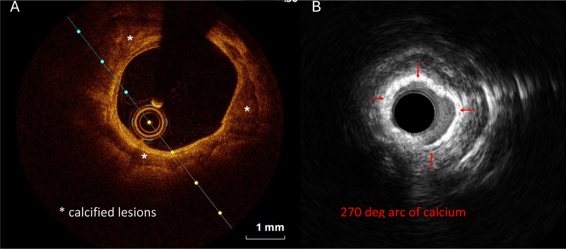
Wang X, Matsumura M, Mintz GS, et al. (2017) In vivo calcium detection by comparing optical coherence tomography, intravascular ultrasound, and angiography. JACC Cardiovasc Imaging 10: 869-879. https://doi.org/10.1016/j.jcmg.2017.05.014 ![]() |
[4] |
Mintz GS (2015) Intravascular imaging of coronary calcification and its clinical implications. JACC Cardiovasc Imaging 8: 461-471. https://doi.org/10.1016/j.jcmg.2015.02.003 ![]() |
[5] |
Shah M, Najam O, Bhindi R, et al. (2021) Calcium modification techniques in complex percutaneous coronary intervention. Circ Cardiovasc Interv 14: e009870. https://doi.org/10.1161/CIRCINTERVENTIONS.120.009870 ![]() |
[6] |
De Maria GL, Scarsini R, Banning AP (2019) Management of calcific coronary artery lesions: Is it time to change our interventional therapeutic approach?. JACC Cardiovasc Interv 12: 1465-1478. https://doi.org/10.1016/j.jcin.2019.03.038 ![]() |
[7] |
Jurado-Román A, Gómez-Menchero A, Rivero-Santana B, et al. (2025) Rotational atherectomy, lithotripsy, or laser for calcified coronary stenosis: the ROLLER COASTR-EPIC22 trial. JACC Cardiovasc Interv 18: 606-618. https://doi.org/10.1016/j.jcin.2024.11.012 ![]() |
[8] |
Mintz GS, Popma JJ, Pichard AD, et al. (1995) Patterns of calcification in coronary artery disease. Circulation 91: 1959-1965. https://doi.org/10.1161/01.CIR.91.7.1959 ![]() |
[9] |
Polonsky TS, McClelland RL, Jorgensen NW, et al. (2010) Coronary artery calcium score and risk classification for coronary heart disease prediction. JAMA 303: 1610-1616. https://doi.org/10.1001/jama.2010.461 ![]() |
[10] |
Miller JM, Rochitte CE, Dewey M, et al. (2008) Diagnostic performance of coronary angiography by 64-row CT. N Engl J Med 359: 2324-2336. https://doi.org/10.1056/NEJMoa0806576 ![]() |
[11] |
Budoff MJ, Dowe D, Jollis JG, et al. (2008) Diagnostic performance of 64-multidetector row coronary computed tomographic angiography for evaluation of coronary artery stenosis in individuals without known coronary artery disease: results from the prospective multicenter ACCURACY (Assessment by Coronary Computed Tomographic Angiography of Individuals Undergoing Invasive Coronary Angiography) trial. J Am Coll Cardiol 52: 1724-1732. https://doi.org/10.1016/j.jacc.2008.07.031 ![]() |
[12] |
Abbara S, Arbab-Zadeh A, Callister TQ, et al. (2009) SCCT guidelines for performance of coronary computed tomographic angiography: a report of the Society of Cardiovascular Computed Tomography Guidelines Committee. J Cardiovasc Comput Tomogr 3: 190-204. https://doi.org/10.1016/j.jcct.2009.03.004 ![]() |
[13] |
Araki M, Park SJ, Dauerman HL, et al. (2022) Optical coherence tomography in coronary atherosclerosis assessment and intervention. Nat Rev Cardiol 19: 684-703. https://doi.org/10.1038/s41569-022-00687-9 ![]() |
[14] |
Kawai K, Sato Y, Hokama JY, et al. (2023) Histology, OCT, and micro-CT evaluation of coronary calcification treated with intravascular lithotripsy: atherosclerotic cadaver study. JACC Cardiovasc Interv 16: 2097-2108. https://doi.org/10.1016/j.jcin.2023.06.021 ![]() |
[15] |
Gruslova AB, Singh S, Hoyt T, et al. (2024) Accuracy of OCT core labs in identifying vulnerable plaque. JACC Cardiovasc Imaging 17: 448-450. https://doi.org/10.1016/j.jcmg.2023.10.005 ![]() |
[16] |
de Graaf MA, Broersen A, Kitslaar PH, et al. (2013) Automatic quantification and characterization of coronary atherosclerosis with computed tomography coronary angiography: cross-correlation with intravascular ultrasound virtual histology. Int J Cardiovasc Imaging 29: 1177-1190. https://doi.org/10.1007/s10554-013-0194-x ![]() |
[17] |
Kim SY, Kim KS, Seung MJ, et al. (2010) The culprit lesion score on multi-detector computed tomography can detect vulnerable coronary artery plaque. Int J Cardiovasc Imaging 26: 245-252. https://doi.org/10.1007/s10554-010-9712-2 ![]() |
[18] |
Mintz GS, Nissen SE, Anderson WD, et al. (2001) American College of Cardiology clinical expert consensus document on standards for acquisition, measurement and reporting of intravascular ultrasound studies (ivus)33. J Am Coll Cardiol 37: 1478-1492. https://doi.org/10.1016/S0735-1097(01)01175-5 ![]() |
[19] |
Zhang M, Matsumura M, Usui E, et al. (2021) Intravascular ultrasound-derived calcium score to predict stent expansion in severely calcified lesions. Circ Cardiovasc Interv 14: e010296. https://doi.org/10.1161/CIRCINTERVENTIONS.120.010296 ![]() |
[20] |
Pu J, Mintz GS, Biro S, et al. (2014) Insights into echo-attenuated plaques, echolucent plaques, and plaques with spotty calcification: novel findings from comparisons among intravascular ultrasound, near-infrared spectroscopy, and pathological histology in 2,294 human coronary artery segments. J Am Coll Cardiol 63: 2220-2233. https://doi.org/10.1016/j.jacc.2014.02.576 ![]() |
[21] |
Mehanna E, Bezerra HG, Prabhu D, et al. (2013) Volumetric characterization of human coronary calcification by frequency-domain optical coherence tomography. Circ J 77: 2334-2340. https://doi.org/10.1253/circj.cj-12-1458 ![]() |
[22] |
Maehara A, Mintz GS, Stone GW (2013) OCT versus IVUS: accuracy versus clinical utility. JACC Cardiovasc Imaging 6: 1105-1107. https://doi.org/10.1016/j.jcmg.2013.05.016 ![]() |
[23] |
Fujino A, Mintz GS, Matsumura M, et al. (2018) A new optical coherence tomography-based calcium scoring system to predict stent underexpansion. EuroIntervention 13: e2182-e2189. https://doi.org/10.4244/EIJ-D-17-00962 ![]() |
[24] |
Généreux P, Madhavan MV, Mintz GS, et al. (2014) Ischemic outcomes after coronary intervention of calcified vessels in acute coronary syndromes. Pooled analysis from the HORIZONS-AMI (Harmonizing Outcomes With Revascularization and Stents in Acute Myocardial Infarction) and ACUITY (Acute Catheterization and Urgent Intervention Triage Strategy) TRIALS. J Am Coll Cardiol 63: 1845-1854. https://doi.org/10.1016/j.jacc.2014.01.034 ![]() |
[25] |
Bourantas CV, Zhang YJ, Garg S, et al. (2014) Prognostic implications of coronary calcification in patients with obstructive coronary artery disease treated by percutaneous coronary intervention: a patient-level pooled analysis of 7 contemporary stent trials. Heart 100: 1158-1164. https://doi.org/10.1136/heartjnl-2013-305180 ![]() |
[26] |
Silvain J, Lattuca B, Beygui F, et al. (2020) Ticagrelor versus clopidogrel in elective percutaneous coronary intervention (ALPHEUS): a randomised, open-label, phase 3b trial. Lancet 396: 1737-1744. https://doi.org/10.1016/S0140-6736(20)32236-4 ![]() |
[27] |
Alfonso F, Macaya C, Goicolea J, et al. (1994) Determinants of coronary compliance in patients with coronary artery disease: an intravascular ultrasound study. J Am Coll Cardiol 23: 879-884. https://doi.org/10.1016/0735-1097(94)90632-7 ![]() |
[28] |
Madhavan MV, Tarigopula M, Mintz GS, et al. (2014) Coronary artery calcification: pathogenesis and prognostic implications. J Am Coll Cardiol 63: 1703-1714. https://doi.org/10.1016/j.jacc.2014.01.017 ![]() |
[29] |
Huisman J, van der Heijden LC, Kok MM, et al. (2017) Two-year outcome after treatment of severely calcified lesions with newer-generation drug-eluting stents in acute coronary syndromes: a patient-level pooled analysis from TWENTE and DUTCH PEERS. J Cardiol 69: 660-665. https://doi.org/10.1016/j.jjcc.2016.06.010 ![]() |
[30] |
Généreux P, Redfors B, Witzenbichler B, et al. (2017) Angiographic predictors of 2-year stent thrombosis in patients receiving drug-eluting stents: insights from the ADAPT-DES study. Catheter Cardiovasc Interv 89: 26-35. https://doi.org/10.1002/ccd.26409 ![]() |
[31] | Kitahara H, Kobayashi Y, Yamaguchi M, et al. (2008) Damage to polymer of undelivered sirolimus-eluting stents. J Invasive Cardiol 20: 130-133. |
[32] |
Lee JB, Mintz GS, Lisauskas JB, et al. (2011) Histopathologic validation of the intravascular ultrasound diagnosis of calcified coronary artery nodules. Am J Cardiol 108: 1547-1551. https://doi.org/10.1016/j.amjcard.2011.07.014 ![]() |
[33] |
Watanabe H, Morimoto T, Natsuaki M, et al. (2022) Comparison of clopidogrel monotherapy after 1 to 2 months of dual antiplatelet therapy with 12 months of dual antiplatelet therapy in patients with acute coronary syndrome: the STOPDAPT-2 ACS randomized clinical trial. JAMA Cardiol 7: 407-417. https://doi.org/10.1001/jamacardio.2021.5244 ![]() |
[34] |
Jaspattananon A, Wongpraparut N, Chotinaiwattarakul C, et al. (2021) A risk predictive model for coronary perforation in patients undergoing percutaneous coronary intervention—APOLLO-XI score. European Heart Journal 42: ehab724.2151. https://doi.org/10.1093/eurheartj/ehab724.2151 ![]() |
[35] |
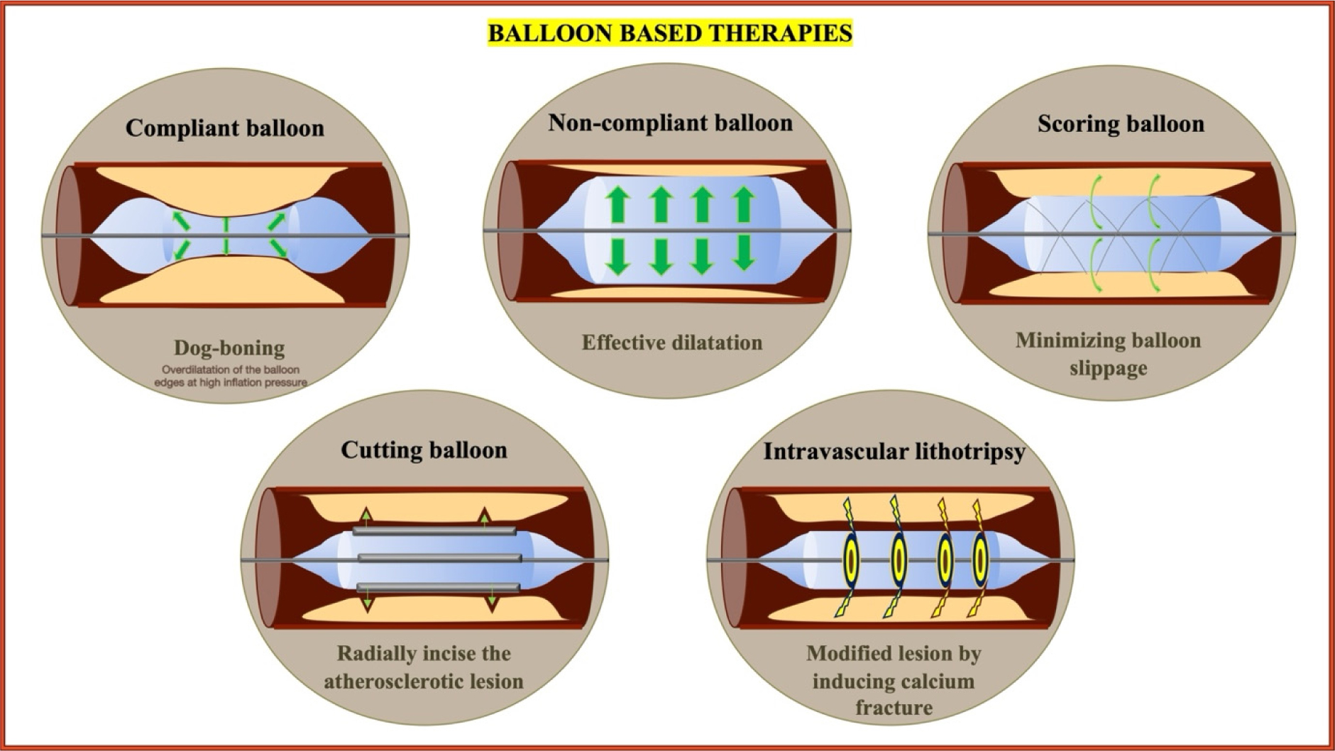
Safian RD, Hoffmann MA, Almany S, et al. (1995) Comparison of coronary angioplasty with compliant and noncompliant balloons (the Angioplasty Compliance Trial). Am J Cardiol 76: 518-520. https://doi.org/10.1016/s0002-9149(99)80143-x ![]() |
[36] |
Kawase Y, Saito N, Watanabe S, et al. (2014) Utility of a scoring balloon for a severely calcified lesion: bench test and finite element analysis. Cardiovasc Interv Ther 29: 134-139. https://doi.org/10.1007/s12928-013-0232-6 ![]() |
[37] |
Liang B, Gu N (2021) Evaluation of the safety and efficacy of coronary intravascular lithotripsy for treatment of severely calcified coronary stenoses: evidence from the serial disrupt CAD trials. Front Cardiovasc Med 8: 724481. https://doi.org/10.3389/fcvm.2021.724481 ![]() |
[38] |
Basavarajaiah S, Ielasi A, Raja W, et al. (2022) Long-term outcomes following intravascular lithotripsy (IVL) for calcified coronary lesions: a real-world multicenter european study. Catheter Cardiovasc Interv 101: 250-260. https://doi.org/10.1002/ccd.30519 ![]() |
[39] |
Gruslova AB, Inanc IH, Cilingiroglu M, et al. (2024) Review of intravascular lithotripsy for treating coronary, peripheral artery, and valve calcifications. Catheter Cardiovasc Interv 103: 295-307. https://doi.org/10.1002/ccd.30933 ![]() |
[40] |
Kereiakes DJ, Di Mario C, Riley RF, et al. (2021) Intravascular lithotripsy for treatment of calcified coronary lesions: patient-level pooled analysis of the disrupt CAD studies. JACC Cardiovasc Interv 14: 1337-1348. https://doi.org/10.1016/j.jcin.2021.04.015 ![]() |
[41] | Dawood M, Elwany M, Abdelgawad H, et al. (2024) Coronary calcifications, the Achilles heel in coronary interventions. Postepy Kardiol Interwencyjnej 20: 1-17. https://doi.org/10.5114/aic.2024.136415 |
[42] |
Safian RD, Feldman T, Muller DW, et al. (2001) Coronary angioplasty and Rotablator atherectomy trial (CARAT): immediate and late results of a prospective multicenter randomized trial. Catheter Cardiovasc Interv 53: 213-220. https://doi.org/10.1002/ccd.1151 ![]() |
[43] |
Sharma SK, Tomey MI, Teirstein PS, et al. (2019) North American expert review of rotational atherectomy. Circ Cardiovasc Interv 12: e007448. https://doi.org/10.1161/CIRCINTERVENTIONS.118.007448 ![]() |
[44] |
Abdel-Wahab M, Richardt G, Joachim Büttner H, et al. (2013) High-speed rotational atherectomy before paclitaxel-eluting stent implantation in complex calcified coronary lesions: the randomized ROTAXUS (Rotational Atherectomy Prior to Taxus Stent Treatment for Complex Native Coronary Artery Disease) trial. JACC Cardiovasc Interv 6: 10-19. https://doi.org/10.1016/j.jcin.2012.07.017 ![]() |
[45] |
Abdel-Wahab M, Toelg R, Byrne RA, et al. (2018) High-speed rotational atherectomy versus modified balloons prior to drug-eluting stent implantation in severely calcified coronary lesions. Circ Cardiovasc Interv 11: e007415. https://doi.org/10.1161/CIRCINTERVENTIONS.118.007415 ![]() |
[46] |
Neumann FJ, Sousa-Uva M, Ahlsson A, et al. (2019) 2018 ESC/EACTS Guidelines on myocardial revascularization. Eur Heart J 40: 87-165. https://doi.org/10.1093/eurheartj/ehy394 ![]() |
[47] |
Dill T, Dietz U, Hamm CW, et al. (2000) A randomized comparison of balloon angioplasty versus rotational atherectomy in complex coronary lesions (COBRA study). Eur Heart J 21: 1759-1766. https://doi.org/10.1053/euhj.2000.2242 ![]() |
[48] |
Mankerious N, Richardt G, Allali A, et al. (2024) Lower revascularization rates after high-speed rotational atherectomy compared to modified balloons in calcified coronary lesions: 5-year outcomes of the randomized PREPARE-CALC trial. Clin Res Cardiol 113: 1051-1059. https://doi.org/10.1007/s00392-024-02434-1 ![]() |
[49] |
Florek K, Bartoszewska E, Biegała S, et al. (2023) Rotational atherectomy, orbital atherectomy, and intravascular lithotripsy comparison for calcified coronary lesions. J Clin Med 12: 7246. https://doi.org/10.3390/jcm12237246 ![]() |
[50] |
Redfors B, Sharma SK, Saito S, et al. (2020) Novel micro crown orbital atherectomy for severe lesion calcification. Circ Cardiovasc Interv 13: e008993. https://doi.org/10.1161/CIRCINTERVENTIONS.120.008993 ![]() |
[51] | Shlofmitz E, Shlofmitz R, Lee MS (2019) Orbital atherectomy: a comprehensive review. Interv Cardiol Clin 8: 161-171. https://doi.org/10.1016/j.iccl.2018.11.006 |
[52] |
Parikh K, Chandra P, Choksi N, et al. (2013) Safety and feasibility of orbital atherectomy for the treatment of calcified coronary lesions: the ORBIT I trial. Catheter Cardiovasc Interv 81: 1134-1139. https://doi.org/10.1002/ccd.24700 ![]() |
[53] |
Chambers JW, Feldman RL, Himmelstein SI, et al. (2014) Pivotal trial to evaluate the safety and efficacy of the orbital atherectomy system in treating de novo, severely calcified coronary lesions (ORBIT II). JACC Cardiovasc Interv 7: 510-518. https://doi.org/10.1016/j.jcin.2014.01.158 ![]() |
[54] |
Lee M, Généreux P, Shlofmitz R, et al. (2017) Orbital atherectomy for treating de novo, severely calcified coronary lesions: 3-year results of the pivotal ORBIT II trial. Cardiovasc Revasc Med 18: 261-264. https://doi.org/10.1016/j.carrev.2017.01.011 ![]() |
[55] | Koike J, Iwasaki Y, Sato T, et al. (2023) Acute and mid-term results of percutaneous coronary intervention for severely calcified coronary artery lesions with orbital atherectomy system. J Invasive Cardiol 35. https://doi.org/10.25270/jic/23.00131 |
[56] |
Rola P, Włodarczak S, Barycki M, et al. (2023) Safety and efficacy of orbital atherectomy in the all-comer population: mid-term results of the Lower Silesian Orbital Atherectomy Registry (LOAR). J Clin Med 12: 5842. https://doi.org/10.3390/jcm12185842 ![]() |
[57] |
Généreux P, Kirtane AJ, Kandzari DE, et al. (2022) Randomized evaluation of vessel preparation with orbital atherectomy prior to drug-eluting stent implantation in severely calcified coronary artery lesions: design and rationale of the ECLIPSE trial. Am Heart J 249: 1-11. https://doi.org/10.1016/j.ahj.2022.03.003 ![]() |
[58] |
Kirtane AJ, Ribichini F (2024) Atherectomy for calcified plaques: orbital for most? Pros and cons. EuroIntervention 20: e627-e629. https://doi.org/10.4244/EIJ-E-24-00014 ![]() |
[59] |
Okamoto N, Egami Y, Nohara H, et al. (2023) Direct comparison of rotational vs orbital atherectomy for calcified lesions guided by optical coherence tomography. JACC Cardiovasc Interv 16: 2125-2136. https://doi.org/10.1016/j.jcin.2023.06.016 ![]() |
[60] |
Shibui T, Tsuchiyama T, Masuda S, et al. (2021) Excimer laser coronary atherectomy prior to paclitaxel-coated balloon angioplasty for de novo coronary artery lesions. Lasers Med Sci 36: 111-117. https://doi.org/10.1007/s10103-020-03019-w ![]() |
[61] |
Tonomura D, Shimada Y, Yamanaka Y, et al. (2022) Laser vaporization of atherothrombotic burden before drug-coated balloon application in ST-segment elevation myocardial infarction: two-year outcomes of the laser-DCB trial. Catheter Cardiovasc Interv 99: 1758-1765. https://doi.org/10.1002/ccd.30149 ![]() |
[62] |
Doolub G, Ly HQ, Marquis-Gravel G (2024) Should rotational atherectomy be used more often in STEMI to treat calcified culprit lesions?. Can J Cardiol 40: 1234-1236. https://doi.org/10.1016/j.cjca.2024.01.021 ![]() |
[63] |
Hemetsberger R, Mankerious N, Muntané-Carol G, et al. (2024) In-hospital outcomes of rotational atherectomy in ST-elevation myocardial infarction: results from the multicentre ROTA-STEMI network. Can J Cardiol 40: 1226-1233. https://doi.org/10.1016/j.cjca.2023.12.018 ![]() |
[64] |
Shahin M, Candreva A, Siegrist PT (2018) Rotational atherectomy in acute STEMI with heavily calcified culprit lesion is a rule breaking solution. Curr Cardiol Rev 14: 213-216. https://doi.org/10.2174/1573403X14666180523084846 ![]() |
[65] | Błaszkiewicz M, Florek K, Zimoch W, et al. (2024) Predictors of periprocedural myocardial infarction after rotational atherectomy. Postepy Kardiol Interwencyjnej 20: 62-66. https://doi.org/10.5114/aic.2024.137419 |
[66] |
Riley RF, Henry TD, Mahmud E, et al. (2020) SCAI position statement on optimal percutaneous coronary interventional therapy for complex coronary artery disease. Catheter Cardiovasc Interv 96: 346-362. https://doi.org/10.1002/ccd.28994 ![]() |
[67] |
Räber L, Mintz GS, Koskinas KC, et al. (2018) Clinical use of intracoronary imaging. Part 1: guidance and optimization of coronary interventions. An expert consensus document of the European Association of Percutaneous Cardiovascular Interventions. Eur Heart J 39: 3281-3300. https://doi.org/10.1093/eurheartj/ehy285 ![]() |
1. | David F. Anderson, James D. Brunner, Gheorghe Craciun, Matthew D. Johnston, On classes of reaction networks and their associated polynomial dynamical systems, 2020, 58, 0259-9791, 1895, 10.1007/s10910-020-01148-9 | |
2. | Juan Kuntz, Philipp Thomas, Guy-Bart Stan, Mauricio Barahona, Stationary Distributions of Continuous-Time Markov Chains: A Review of Theory and Truncation-Based Approximations, 2021, 63, 0036-1445, 3, 10.1137/19M1289625 | |
3. | Daniele Cappelletti, Andrés Ortiz-Muñoz, David F. Anderson, Erik Winfree, Stochastic chemical reaction networks for robustly approximating arbitrary probability distributions, 2020, 801, 03043975, 64, 10.1016/j.tcs.2019.08.013 | |
4. | Daniele Cappelletti, Badal Joshi, Transition graph decomposition for complex balanced reaction networks with non-mass-action kinetics, 2022, 19, 1551-0018, 7649, 10.3934/mbe.2022359 | |
5. | Ander Movilla Miangolarra, Michele Castellana, On Non-ideal Chemical-Reaction Networks and Phase Separation, 2023, 190, 0022-4715, 10.1007/s10955-022-03037-8 | |
6. | David F. Anderson, Tung D. Nguyen, Deficiency zero for random reaction networks under a stochastic block model framework, 2021, 59, 0259-9791, 2063, 10.1007/s10910-021-01278-8 | |
7. | Linard Hoessly, Stationary distributions via decomposition of stochastic reaction networks, 2021, 82, 0303-6812, 10.1007/s00285-021-01620-3 | |
8. | David F. Anderson, Tung D. Nguyen, Prevalence of deficiency-zero reaction networks in an Erdös–Rényi framework, 2022, 59, 0021-9002, 384, 10.1017/jpr.2021.65 | |
9. | Beatriz Pascual-Escudero, Linard Hoessly, An Algebraic Approach to Product-form Stationary Distributions for Some Reaction Networks, 2022, 21, 1536-0040, 588, 10.1137/21M1401498 | |
10. | Nidhi Kaihnsa, Tung Nguyen, Anne Shiu, Absolute concentration robustness and multistationarity in reaction networks: Conditions for coexistence, 2024, 35, 0956-7925, 566, 10.1017/S0956792523000335 | |
11. | Badal Joshi, Nidhi Kaihnsa, Tung D. Nguyen, Anne Shiu, Prevalence of Multistationarity and Absolute Concentration Robustness in Reaction Networks, 2023, 83, 0036-1399, 2260, 10.1137/23M1549316 | |
12. | David F. Anderson, Daniele Cappelletti, Wai-Tong Louis Fan, Jinsu Kim, A New Path Method for Exponential Ergodicity of Markov Processes on Zd, with Applications to Stochastic Reaction Networks, 2025, 24, 1536-0040, 1668, 10.1137/24M1665933 |