The consumption and usage of polyethylene terephthalate (PET) bottles have significantly increased in recent years, necessitating action to mitigate their environmental impact. Recycling programs offer a viable solution to address this impact within the PET industry. Therefore, adopting a circular economy approach is appropriate for incorporating recycling initiatives. Nevertheless, it is crucial not to overlook the financial aspects of the supply chain. This paper proposed a bi-level model to address both the financial and environmental concerns of a circular economy supply chain. At the upper level, a recycling company (the leader) aimd to establish PET bottle collection facilities, set prices for each kilogram of PET received, and manage the transportation of collected PET to the treatment plant. At the lower level of the bi-level problem, persons (the followers) decided whether to recycle or not. They received economic incentives based on the amount deposited at the collection facilities, but this came with associated travel costs. The leader's objective was to maximize the profit of the recycling program, assuming the sale of recycled PET. Meanwhile, followers aimed to recycle if it was economically viable for them. To solve this problem, a matheuristic algorithm was proposed, which hybridized a greedy random adaptive search procedure with an exact routing process. The matheuristic managed solutions at the leader level, while followers' responses were derived by exploiting the problem's structure. A case study derived from Mexico City was solved, and practical managerial insights were provided. Sensitivity analysis revealed crucial aspects that should not be overlooked when implementing such a recycling program.
Citation: Carlos Corpus, Ali Zahedi, Eva Selene Hernández-Gress, José-Fernando Camacho-Vallejo. A bi-level optimization model for PET bottle recycling within a circular economy supply chain[J]. AIMS Environmental Science, 2025, 12(2): 223-251. doi: 10.3934/environsci.2025010
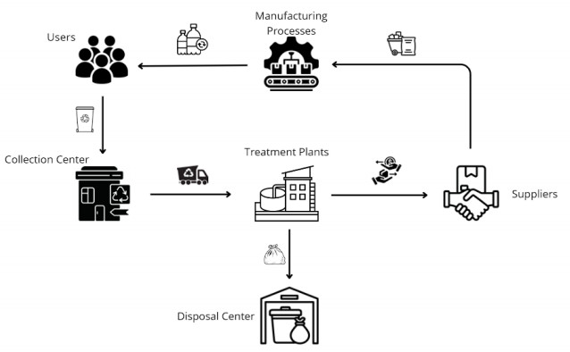
The consumption and usage of polyethylene terephthalate (PET) bottles have significantly increased in recent years, necessitating action to mitigate their environmental impact. Recycling programs offer a viable solution to address this impact within the PET industry. Therefore, adopting a circular economy approach is appropriate for incorporating recycling initiatives. Nevertheless, it is crucial not to overlook the financial aspects of the supply chain. This paper proposed a bi-level model to address both the financial and environmental concerns of a circular economy supply chain. At the upper level, a recycling company (the leader) aimd to establish PET bottle collection facilities, set prices for each kilogram of PET received, and manage the transportation of collected PET to the treatment plant. At the lower level of the bi-level problem, persons (the followers) decided whether to recycle or not. They received economic incentives based on the amount deposited at the collection facilities, but this came with associated travel costs. The leader's objective was to maximize the profit of the recycling program, assuming the sale of recycled PET. Meanwhile, followers aimed to recycle if it was economically viable for them. To solve this problem, a matheuristic algorithm was proposed, which hybridized a greedy random adaptive search procedure with an exact routing process. The matheuristic managed solutions at the leader level, while followers' responses were derived by exploiting the problem's structure. A case study derived from Mexico City was solved, and practical managerial insights were provided. Sensitivity analysis revealed crucial aspects that should not be overlooked when implementing such a recycling program.

| [1] |
Welle F (2011) Twenty years of pet bottle to bottle recycling—an overview. Resour Conserv Recycl 55: 865–875. https://doi.org/10.1016/j.resconrec.2011.04.009 doi: 10.1016/j.resconrec.2011.04.009

|
| [2] |
Kutralam-Muniasamy G, Shruti V C, Pérez-Guevara F (2023) Citizen involvement in reducing end-of-life product waste in mexico city. Sustain Prod Consump 41: 167–178. https://doi.org/10.1016/j.spc.2023.08.010 doi: 10.1016/j.spc.2023.08.010
|
| [3] | Vlad I M, Toma E (2022) Overview on the key figures with impact on the circular economy through the life cycle of plastics. Mater Plast 59. https://doi.org/10.37358/MP.22.2.5594 |
| [4] | Hotspot H C (2021) Waste management in the latam region: business opportunities for the netherlands in waste/circular economy sector in eight countries of latin america. The Netherlands Enterprise Agency (RVO), The Hague. |
| [5] |
Gutierrez Galicia F, Coria Paez A L, Tejeida Padilla R (2019) A study and factor identification of municipal solid waste management in mexico city. Sustainability 11: 6305. https://doi.org/10.3390/su11226305 doi: 10.3390/su11226305
|
| [6] |
Olay-Romero E, Turcott-Cervantes D E, del Consuelo Hernández-Berriel M, et al. (2020) Technical indicators to improve municipal solid waste management in developing countries: A case in mexico. Waste Manage 107: 201–210. https://doi.org/10.1016/j.wasman.2020.03.039 doi: 10.1016/j.wasman.2020.03.039
|
| [7] | Esposito M, Tse T, Soufani K (2017) Is the circular economy a new fast-expanding market? Thunderbird Int Bus Rev 59: 9–14. https://doi.org/10.1002/tie.21764 |
| [8] |
Abad-Segura E, Fuente A B, González-Zamar M D, et al. (2020) Effects of circular economy policies on the environment and sustainable growth: Worldwide research. Sustainability 12: 5792. https://doi.org/10.3390/su12145792 doi: 10.3390/su12145792
|
| [9] |
Gallego-Schmid A, Chen H M, Sharmina M, et al. (2020) Links between circular economy and climate change mitigation in the built environment. J Clean Prod 260: 121115. https://doi.org/10.1016/j.jclepro.2020.121115 doi: 10.1016/j.jclepro.2020.121115
|
| [10] |
Georgescu I, Kinnunen J, Androniceanu A M (2022) Empirical evidence on circular economy and economic development in europe: a panel approach. J Bus Econ Manag 23: 199–217. https://doi.org/10.3846/jbem.2022.16050 doi: 10.3846/jbem.2022.16050
|
| [11] |
Bing X, de Keizer M, Bloemhof-Ruwaard J M, et al.(2014) Vehicle routing for the eco-efficient collection of household plastic waste. Waste manage 34: 719–729. https://doi.org/10.1016/j.wasman.2014.01.018 doi: 10.1016/j.wasman.2014.01.018
|
| [12] |
Marampoutis I, Vinot M, Trilling L (2022) Multi-objective vehicle routing problem with flexible scheduling for the collection of refillable glass bottles: A case study. EURO J Decis Process 10: 100011. https://doi.org/10.1016/j.ejdp.2021.100011 doi: 10.1016/j.ejdp.2021.100011
|
| [13] | McDonough W, Braungart M (2010) Cradle to cradle: Remaking the way we make things. North point press. |
| [14] |
Shen L, Worrell E, Patel M K (2010) Open-loop recycling: A lca case study of pet bottle-to-fibre recycling. Resour Conserv Recycl 55: 34–52. https://doi.org/10.1016/j.resconrec.2010.06.014 doi: 10.1016/j.resconrec.2010.06.014
|
| [15] |
Stallkamp C, Hennig M, Volk R, et al. (2024) Pyrolysis of mixed engineering plastics: Economic challenges for automotive plastic waste. Waste Manage 176: 105–116. https://doi.org/10.1016/j.wasman.2024.01.035 doi: 10.1016/j.wasman.2024.01.035
|
| [16] |
van Langen S K, Passaro R (2021) The dutch green deals policy and its applicability to circular economy policies. Sustainability 13: 11683. https://doi.org/10.3390/su132111683 doi: 10.3390/su132111683
|
| [17] | Cámara-Creixell J, Scheel-Mayenberger C (2019) Petstar pet bottle-to-bottle recycling system, a zero-waste circular economy business model. Towards Zero Waste Circular Economy Boost Waste Resour 191–213. |
| [18] |
Pinter E, Welle F, Mayrhofer E, et al. (2021) Circularity study on pet bottle-to-bottle recycling. Sustainability 13: 7370. https://doi.org/10.3390/su13137370 doi: 10.3390/su13137370
|
| [19] |
Lonca G, Lesage P, Majeau-Bettez G, et al. (2020) Assessing scaling effects of circular economy strategies: A case study on plastic bottle closed-loop recycling in the usa pet market. Resour Conserv Recycl 162: 105013. https://doi.org/10.1016/j.resconrec.2020.105013 doi: 10.1016/j.resconrec.2020.105013
|
| [20] |
Benyathiar P, Kumar P, Carpenter G, et al. (2022) Polyethylene terephthalate (pet) bottle-to-bottle recycling for the beverage industry: a review. Polymers 14: 2366. https://doi.org/10.3390/polym14122366 doi: 10.3390/polym14122366
|
| [21] | Zapata Bravo Á, Vieira Escobar V, Zapata-Domínguez Á, et al. (2021) The circular economy of pet bottles in colombia. Cuadernos de Administración (Universidad del Valle) 37. https://doi.org/10.25100/cdea.v37i70.10912 |
| [22] |
Gall M, Schweighuber A, Buchberger W, et al. (2020) Plastic bottle cap recycling—characterization of recyclate composition and opportunities for design for circularity. Sustainability 12: 10378. https://doi.org/10.3390/su122410378 doi: 10.3390/su122410378
|
| [23] |
Gracida-Alvarez U R, Xu H, Benavides P T, et al. (2023) Circular economy sustainability analysis framework for plastics: application for poly (ethylene terephthalate)(pet). ACS Sustainable Chemistry & Engineering 11: 514–524. https://doi.org/10.1021/acssuschemeng.2c04626 doi: 10.1021/acssuschemeng.2c04626
|
| [24] |
Wang Y, Gu Y, Wu Y, et al. (2020) Performance simulation and policy optimization of waste polyethylene terephthalate bottle recycling system in china. Resour Conserv Recycl 162: 105014. https://doi.org/10.1016/j.resconrec.2020.105014 doi: 10.1016/j.resconrec.2020.105014
|
| [25] |
Ayeleru O O, Dlova S, Akinribide O J, et al. (2020) Challenges of plastic waste generation and management in sub-saharan africa: A review. Waste Manage 110: 24–42. https://doi.org/10.1016/j.wasman.2020.04.017 doi: 10.1016/j.wasman.2020.04.017
|
| [26] |
Amirudin A, Inoue C, Grause G (2023) Assessment of factors influencing indonesian residents’ intention to use a deposit–refund scheme for pet bottle waste. Circular Economy 2: 100061. https://doi.org/10.1016/j.cec.2023.100061 doi: 10.1016/j.cec.2023.100061
|
| [27] |
Oliveira Neto G C, de Araujo S A, Gomes R A, et al. (2023) Simulation of electronic waste reverse chains for the sao paulo circular economy: An artificial intelligence-based approach for economic and environmental optimizations. Sensors 23: 9046. https://doi.org/10.3390/s23229046 doi: 10.3390/s23229046
|
| [28] |
Rahmanifar G, Mohammadi M, Sherafat A, et al. (2023) Heuristic approaches to address vehicle routing problem in the iot-based waste management system. Expert Syst Appl 220: 119708. https://doi.org/10.1016/j.eswa.2023.119708 doi: 10.1016/j.eswa.2023.119708
|
| [29] | Rekabi S, Sazvar Z, Tavakkoli-Moghaddam R (2022) A green vehicle routing problem in the solid waste network design with vehicle and technology compatibility. Comput Sci Eng 2: 299–309. |
| [30] |
Ng T S A, Mah A X Y, Zhao K (2024) Towards a circular economy with waste-to-resource system optimization. Nav Res Logist 71: 553–574. https://doi.org/10.1002/nav.22163 doi: 10.1002/nav.22163
|
| [31] |
Cao C, Liu J, Liu Y, et al. (2023) Digital twin-driven robust bi-level optimisation model for covid-19 medical waste location-transport under circular economy. Comput Ind Eng 186: 109107. https://doi.org/10.1016/j.cie.2023.109107 doi: 10.1016/j.cie.2023.109107
|
| [32] | Kokossis A, Melampianakis E (2022) A game-theoretical approach for the analysis of waste treatment and circular economy networks. In Comput Aided Chem Eng 51: 1657–1662. https://doi.org/10.1016/B978-0-323-95879-0.50277-0 |
| [33] |
Huang Y, Xu J (2022) Bi-level multi-objective programming approach for bioenergy production optimization towards co-digestion of kitchen waste and rice straw. Fuel 316: 123117. https://doi.org/10.1016/j.fuel.2021.123117 doi: 10.1016/j.fuel.2021.123117
|
| [34] |
Safder U, Tariq S, Yoo C K (2022) Multilevel optimization framework to support self-sustainability of industrial processes for energy/material recovery using circular integration concept. Appl Energy 324: 119685. https://doi.org/10.1016/j.apenergy.2022.119685 doi: 10.1016/j.apenergy.2022.119685
|
| [35] | Alimohammadi M, Behnamian J (2024) Supporting circular economy through using digital transformation in sustainable pharmaceutical reverse logistics: Multi-objective bi-level modeling. Process Integr Optim Sustain 1–26. https://doi.org/10.1007/s41660-024-00460-0 |
| [36] |
Calvete H I, Gal C (2007) Linear bilevel multi-follower programming with independent followers. J Glob Optim 39: 409–417. https://doi.org/10.1007/s10898-007-9144-2 doi: 10.1007/s10898-007-9144-2
|
| [37] | Dempe S, Zemkoho A (2020) Bilevel optimization. In Springer optimization and its applications 161. Springer. https://doi.org/10.1007/978-3-030-52119-6 |
| [38] |
Boschetti M A, Maniezzo V (2022) Matheuristics: using mathematics for heuristic design. 4OR 20: 173–208. https://doi.org/10.1007/s10288-022-00510-8 doi: 10.1007/s10288-022-00510-8
|
| [39] | Camacho-Vallejo J F, Corpus C, Villegas J G (2023) Metaheuristics for bilevel optimization: A comprehensive review. Comput Oper Res 106410. https://doi.org/10.1016/j.cor.2023.106410 |
| [40] | Resende M G C, Ribeiro C C (2016) Optimization by GRASP. Springer. https://doi.org/10.1007/978-1-4939-6530-4 |
| [41] | Zaleta J (2024) ¿cuánto dinero puedes ganar reciclando? esto es lo que vale el kilo de pet en méxico? https://heraldodemexico.com.mx/estilo-de-vida/2024/2/5/cuanto-dinero-puedes-ganar-reciclando-esto-es-lo-que-vale-el-kilo-de-pet-en-mexico-575356.html, 2024. Accessed: 2024-07-15. |
| [42] | Álvarez D (2024) Costo de materiales reciclables a la baja. https://www.diariodequeretaro.com.mx/finanzas/costo-de-materiales-reciclables-a-la-baja-10186587.html#:~:text=El%20precio%20com%C3%BAn%20para%20el,y%20de%20segunda%20en%20100., 2024. Accessed: 2024-07-15. |
| [43] | ULINE. Contenedor plegable para carga a granel - 32 x 30 x 34", capacidad de 1,500 lb. https://es.uline.mx/Product/Detail/H-4051/Bulk-Containers/Collapsible-Bulk-Container-32-x-30-x-34-1500-Capacity?pricode=WB7091&gadtype=pla&id=H-4051&gad_source=1&gclid=Cj0KCQjw7ZO0BhDYARIsAFttkCinP4LOAdO0G_KuTh4Xn_gXz5KsloY0fRvemZJlN0svbQeK8OorZQIaAoAZEALw_wcB, 2024. Accessed: 2024-07-15. |
| [44] | Educa verde. https://educa-verde.ecoce.mx, 2024. Accessed: 2024-07-15. |


Figures(9)

Carlos Corpus, Ali Zahedi, Eva Selene Hernández-Gress, José-Fernando Camacho-Vallejo. A bi-level optimization model for PET bottle recycling within a circular economy supply chain[J]. AIMS Environmental Science, 2025, 12(2): 223-251. doi: 10.3934/environsci.2025010


 DownLoad: