Nowadays, traditional machine learning methods for building predictive models of credit card customer churn are no longer sufficient for effective customer management. Additionally, interpreting these models has become essential. This study aims to balance the data using sampling techniques to forecast whether a customer will churn, combine machine learning methods to build a comprehensive customer churn prediction model, and select the model with the best performance. The optimal model is then interpreted using the Shapley Additive exPlanations (SHAP) values method to analyze the correlation between each independent variable and customer churn. Finally, the causal impacts of these variables on customer churn are explored using the R-learner causal inference method. The results show that the complete customer churn prediction model using Extreme Gradient Boosting (XGBoost) achieved significant performance, with accuracy, precision, recall, F1 score, and area under the curve (AUC) all reaching 97%. The SHAP values method and causal inference method demonstrate that several variables, such as the customer's total number of transactions, the total transaction amount, the total number of bank products, and the changes in both the amount and the number of transactions from the fourth quarter to the first quarter, have an impact on customer churn, providing a theoretical foundation for customer management.
Citation: Ying Li, Keyue Yan. Prediction of bank credit customers churn based on machine learning and interpretability analysis[J]. Data Science in Finance and Economics, 2025, 5(1): 19-34. doi: 10.3934/DSFE.2025002
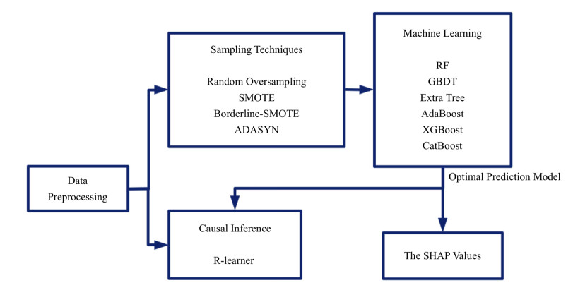
Nowadays, traditional machine learning methods for building predictive models of credit card customer churn are no longer sufficient for effective customer management. Additionally, interpreting these models has become essential. This study aims to balance the data using sampling techniques to forecast whether a customer will churn, combine machine learning methods to build a comprehensive customer churn prediction model, and select the model with the best performance. The optimal model is then interpreted using the Shapley Additive exPlanations (SHAP) values method to analyze the correlation between each independent variable and customer churn. Finally, the causal impacts of these variables on customer churn are explored using the R-learner causal inference method. The results show that the complete customer churn prediction model using Extreme Gradient Boosting (XGBoost) achieved significant performance, with accuracy, precision, recall, F1 score, and area under the curve (AUC) all reaching 97%. The SHAP values method and causal inference method demonstrate that several variables, such as the customer's total number of transactions, the total transaction amount, the total number of bank products, and the changes in both the amount and the number of transactions from the fourth quarter to the first quarter, have an impact on customer churn, providing a theoretical foundation for customer management.

| [1] |
Akın P (2023) A new hybrid approach based on genetic algorithm and support vector machine methods for hyperparameter optimization in synthetic minority over-sampling technique (SMOTE). AIMS Math 8: 9400–9415. https://doi.org/10.3934/math.2023473 doi: 10.3934/math.2023473

|
| [2] |
Alam TM, Shaukat K, Hameed IA, et al. (2020) An Investigation of Credit Card Default Prediction in the Imbalanced Datasets. IEEE Access 8: 201173–201198. https://doi.org/10.1109/access.2020.3033784 doi: 10.1109/access.2020.3033784
|
| [3] |
Alfaiz NS, Fati SM (2022) Enhanced Credit Card Fraud Detection Model Using Machine Learning. Electronics 11: 662. https://doi.org/10.3390/electronics11040662 doi: 10.3390/electronics11040662
|
| [4] |
AL-Najjar D, Al-Rousan N, AL-Najjar H (2022) Machine learning to develop credit card customer churn prediction. J Theor Appl El Comm 17: 1529–1542. https://doi.org/10.3390/jtaer17040077 doi: 10.3390/jtaer17040077
|
| [5] | Bank Churners (2022) Kaggle. Available from: http://www.kaggle.com/competitions/bank-churners/overview. |
| [6] |
Butaru F, Chen Q, Clark B, et al. (2016) Risk and Risk Management in the Credit Card Industry. J Bank Financ 72: 218–239. https://doi.org/10.1016/j.jbankfin.2016.07.015 doi: 10.1016/j.jbankfin.2016.07.015
|
| [7] |
Chang V, Hall K, Xu Qa, et al. (2024) Prediction of Customer Churn Behavior in the Telecommunication Industry Using Machine Learning Models. Algorithms 17: 231. https://doi.org/10.3390/a17060231 doi: 10.3390/a17060231
|
| [8] |
Chen K, Meng X (2020) Interpretation and Understanding in Machine Learning. J Comput Res Dev 57: 1971–1986. https://doi.org/10.7544/issn1000-1239.2020.20190456 doi: 10.7544/issn1000-1239.2020.20190456
|
| [9] |
de Lima Lemos RA, Silva TC, Tabak BM (2022) Propension to customer churn in a financial institution: a machine learning approach. Neural Comput Appl 34: 11751–11768. https://doi.org/10.1007/s00521-022-07067-x doi: 10.1007/s00521-022-07067-x
|
| [10] |
Dube L, Verster T (2023) Enhancing classification performance in imbalanced datasets: A comparative analysis of machine learning models. Data Sci Financ Econ 3: 354–379. https://doi.org/10.3934/dsfe.2023021 doi: 10.3934/dsfe.2023021
|
| [11] |
Erfanian S, Zhou Y, Razzaq A, et al. (2022) Predicting Bitcoin (BTC) Price in the Context of Economic Theories: A Machine Learning Approach. Entropy 24: 1487. https://doi.org/10.3390/e24101487 doi: 10.3390/e24101487
|
| [12] | Facure M (2023) Causal Inference in Python. O'Reilly Media, Inc. |
| [13] |
Feuerriegel S, Frauen D, Melnychuk V, et al. (2024) Causal machine learning for predicting treatment outcomes. Nat Med 30: 958–968. https://doi.org/10.1038/s41591-024-02902-1 doi: 10.1038/s41591-024-02902-1
|
| [14] |
Gebreyesus Y, Dalton D, Nixon S, et al. (2023) Machine Learning for Data Center Optimizations: Feature Selection Using Shapley Additive exPlanation (SHAP). Future Internet 15: 88. https://doi.org/10.3390/fi15030088 doi: 10.3390/fi15030088
|
| [15] |
Gu Q, Song S, Zhang X, et al. (2023) Personal Credit Risk Assessment Based on Improved BS-Stacking. Oper Res Manage Sci 32: 137–144. https://doi.org/10.12005/orms.2023.0262 doi: 10.12005/orms.2023.0262
|
| [16] |
Guo K, Fan H (2024) Research on AdaFocal-XGBoost Integrated Credit Scoring Model Based on Unbalanced Data. Stat Appl 13: 2204–2214. https://doi.org/10.12677/sa.2024.136214 doi: 10.12677/sa.2024.136214
|
| [17] |
Janiesch C, Zschech P, Heinrich K (2021) Machine learning and deep learning. Electron Mark 31: 685–695. https://doi.org/10.1007/s12525-021-00475-2 doi: 10.1007/s12525-021-00475-2
|
| [18] |
Jiang T (2022) Mediating Effects and Moderating Effects in Causal Inference. China Ind Econ 5: 100–120. https://doi.org/10.19581/j.cnki.ciejournal.2022.05.005 doi: 10.19581/j.cnki.ciejournal.2022.05.005
|
| [19] |
Künzel SR, Sekhon JS, Bickel PJ, et al. (2019) Metalearners for estimating heterogeneous treatment effects using machine learning. P Natl Acad Sci 116: 4156–4165. https://doi.org/10.1073/pnas.1804597116 doi: 10.1073/pnas.1804597116
|
| [20] |
Lalwani P, Mishra MK, Chadha JS, et al. (2022) Customer churn prediction system: a machine learning approach. Computing 104: 271–294. https://doi.org/10.1007/s00607-021-00908-y doi: 10.1007/s00607-021-00908-y
|
| [21] |
Li J, Xiong R, Lan Y, et al. (2023) Overview of the Frontier Progress of Causal Machine Learning. J Comput Res Dev 60: 59–84. https://doi.org/10.7544/issn1000-1239.202110780 doi: 10.7544/issn1000-1239.202110780
|
| [22] |
Li Y, Yan K (2023) Prediction of Barrier Option Price Based on Antithetic Monte Carlo and Machine Learning Methods. Cloud Comput Data Sci 4: 77–86. https://doi.org/10.37256/ccds.4120232110 doi: 10.37256/ccds.4120232110
|
| [23] | Molak A (2023) Causal Inference and Discovery in Python. Packt Publishing Ltd. |
| [24] |
Peng K, Peng Y, Li W (2023) Research on customer churn prediction and model interpretability analysis. PLOS ONE 18: e0289724. https://doi.org/10.1371/journal.pone.0289724 doi: 10.1371/journal.pone.0289724
|
| [25] |
Pudjihartono N, Fadason T, Kempa-Liehr AW, et al. (2022) A Review of Feature Selection Methods for Machine Learning-Based Disease Risk Prediction. Front Bioinform 2: 927312. https://doi.org/10.3389/fbinf.2022.927312 doi: 10.3389/fbinf.2022.927312
|
| [26] |
Siddiqui N, Haque MA, Khan SMS, et al. (2024) Different ML-based strategies for customer churn prediction in banking sector. J Data Inf Manage 6: 217–234. https://doi.org/10.1007/s42488-024-00126-z doi: 10.1007/s42488-024-00126-z
|
| [27] |
Wu M, Mao Z, Wang D (2024) Shapley Value and its Application. Math Model Appl 13: 110–119. https://doi.org/10.19943/j.2095-3070.jmmia.2024.01.13 doi: 10.19943/j.2095-3070.jmmia.2024.01.13
|
| [28] |
Yan K, Li Y (2024) Machine learning-based analysis of volatility quantitative investment strategies for American financial stocks. Quant Financ Econ 8: 364–386. https://doi.org/10.3934/QFE.2024014 doi: 10.3934/QFE.2024014
|
| [29] |
Yan K, Wang Y, Li Y (2023) Enhanced Bollinger Band Stock Quantitative Trading Strategy Based on Random Forest. Artif Intell Evol 4: 22–33. https://doi.org/10.37256/aie.4120231991 doi: 10.37256/aie.4120231991
|
| [30] | Zhang N, Zheng Y, Duan C (2024) Bank Customer Churn Prediction based on Random Forest Algorithm. In Proceedings of the 5th International Conference on Computer Information and Big Data Applications : 1031–1035. https://doi.org/10.1145/3671151.3671331 |


Figures(6) / Tables(3)
Ying Li, Keyue Yan. Prediction of bank credit customers churn based on machine learning and interpretability analysis[J]. Data Science in Finance and Economics, 2025, 5(1): 19-34. doi: 10.3934/DSFE.2025002


 DownLoad: