Understanding mathematical identity is critical, thereby reflecting a student's relationship with mathematics and their academic performance. Gender, socioeconomic status, family education level, and personal beliefs may contribute to shaping this identity, especially in non-Western countries such as Turkey. This study aims to investigate the role of gender, socioeconomic status, family education level, mathematics achievement, mathematical beliefs, attitudes towards mathematics, and mathematics motivation as predictors of mathematical identity among Turkish elementary school students. The study, which employed a survey research design, involved 520 elementary school students. Data were collected through five instruments, including a self-description form and a demographic questionnaire. The data were analyzed using multiple regression analyses to explore relationships between the variables. The results revealed that the father's education level, mathematical beliefs, attitudes towards mathematics, and motivation for mathematics significantly predicted the mathematical identity. However, gender, socioeconomic status, maternal education level, and mathematics achievement did not considerably affect the mathematical identity. These findings suggest that intrinsic factors such as beliefs and motivation play a more substantial role in the development of mathematical identity than demographic factors. The study highlights the importance of fostering positive mathematical attitudes and motivation to strengthen a student's mathematical identity. Further research should examine the underlying mechanisms between these predictors and mathematical identity, thereby considering cross-cultural comparisons and longitudinal data to understand how these relationships evolve.
Citation: Hakan Ulum. Understanding Turkish students' mathematical identity: Mathematics achievement, beliefs, attitudes and motivation[J]. STEM Education, 2025, 5(1): 89-108. doi: 10.3934/steme.2025005
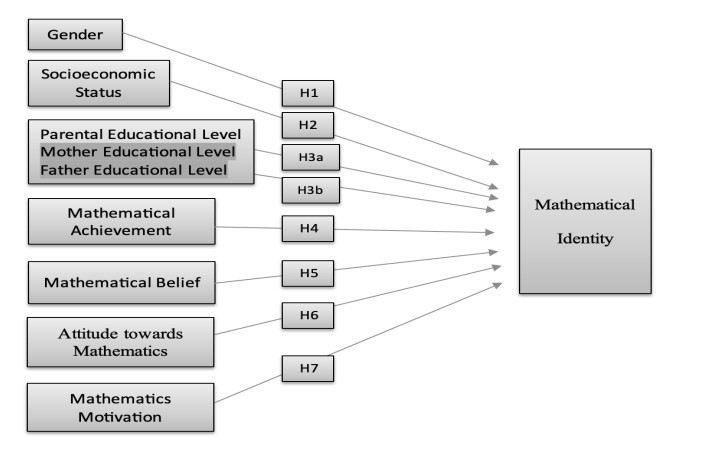
Understanding mathematical identity is critical, thereby reflecting a student's relationship with mathematics and their academic performance. Gender, socioeconomic status, family education level, and personal beliefs may contribute to shaping this identity, especially in non-Western countries such as Turkey. This study aims to investigate the role of gender, socioeconomic status, family education level, mathematics achievement, mathematical beliefs, attitudes towards mathematics, and mathematics motivation as predictors of mathematical identity among Turkish elementary school students. The study, which employed a survey research design, involved 520 elementary school students. Data were collected through five instruments, including a self-description form and a demographic questionnaire. The data were analyzed using multiple regression analyses to explore relationships between the variables. The results revealed that the father's education level, mathematical beliefs, attitudes towards mathematics, and motivation for mathematics significantly predicted the mathematical identity. However, gender, socioeconomic status, maternal education level, and mathematics achievement did not considerably affect the mathematical identity. These findings suggest that intrinsic factors such as beliefs and motivation play a more substantial role in the development of mathematical identity than demographic factors. The study highlights the importance of fostering positive mathematical attitudes and motivation to strengthen a student's mathematical identity. Further research should examine the underlying mechanisms between these predictors and mathematical identity, thereby considering cross-cultural comparisons and longitudinal data to understand how these relationships evolve.

| [1] | Allen, K. and Schnell, K., Developing mathematics identity. Mathematics Teaching in the Middle School, 2016, 21(7): 398–405. |
| [2] |
Axelsson, G.B., Mathematical identity in women: The concept, its components, and relationship to educative ability, achievement, and family support. International Journal of Lifelong Education, 2009, 28(3): 383–406. https://doi.org/10.1080/02601370902757066 doi: 10.1080/02601370902757066

|
| [3] |
Bentler, P.M. and Bonett, D.G., Significance tests and goodness of fit in the analysis of covariance structures. Psychological Bulletin, 1980, 88(3): 588–606. https://doi.org/10.1037/0033-2909.88.3.588 doi: 10.1037/0033-2909.88.3.588
|
| [4] |
Bishop, J.P., She's always been the smart one. I've always been the dumb one: Identities in the mathematics classroom. Journal for Research in Mathematics Education, 2012, 43(1): 34–74. https://doi.org/10.5951/jresematheduc.43.1.0034 doi: 10.5951/jresematheduc.43.1.0034
|
| [5] |
Bohrnstedt, G.W., Cohen, E.D., Yee, D. and Broer, M., Mathematics identity and discrepancies between self-and reflected appraisals: Their relationships with grade 12 mathematics achievement using new evidence from a US national study. Social Psychology of Education, 2021, 24: 763–788. https://doi.org/10.1007/s11218-021-09647-6 doi: 10.1007/s11218-021-09647-6
|
| [6] |
Chen, X., Leung, F.K. and She, J., Dimensions of students' views of classroom teaching and attitudes towards mathematics: A multi-group analysis between genders based on structural equation models. Studies in Educational Evaluation, 2023, 78: 101289. https://doi.org/10.1016/j.stueduc.2023.101289 doi: 10.1016/j.stueduc.2023.101289
|
| [7] |
Côté, J., Identity studies: How close are we to developing a social science of identity? An appraisal of the field. Identity, 2006, 6(1): 3–25. https://doi.org/10.1207/s1532706xid0601_2 doi: 10.1207/s1532706xid0601_2
|
| [8] |
Cragg, L., Keeble, S., Richardson, S., Roome, H.E. and Gilmore, C., Direct and indirect influences of executive functions on mathematics achievement. Cognition, 2017,162: 12–26. https://doi.org/10.1016/j.cognition.2017.01.014 doi: 10.1016/j.cognition.2017.01.014
|
| [9] | Cribbs, J.D. and Piatek-Jimenez, K., Exploring how gender, self-identified personality attributes, mathematics identity, and gender identification contribute to college students' STEM career goals. International Journal of Innovation in Science and Mathematics Education, 2021, 29(2): 47–59. |
| [10] |
Cribbs, J.D. and Utley, J., Mathematics identity instrument development for fifth through twelfth grade students. Mathematics Education Research Journal, 2023, 1–23. https://doi.org/10.1007/s13394-023-00472-6 doi: 10.1007/s13394-023-00472-6
|
| [11] |
Cribbs, J.D., Hazari, Z., Sonnert, G. and Sadler, P.M., Establishing an explanatory model for mathematics identity. Child Development, 2015, 86(4): 1048–1062. https://doi.org/10.1111/cdev.12363 doi: 10.1111/cdev.12363
|
| [12] |
Cribbs, J., Huang, X. and Piatek-Jimenez, K., Relations of mathematics mindset, mathematics anxiety, mathematics identity, and mathematics self-efficacy to STEM career choice: A structural equation modeling approach. School Science and Mathematics, 2021,121(5): 275–287. https://doi.org/10.1111/ssm.12423 doi: 10.1111/ssm.12423
|
| [13] |
Darragh, L., Identity research in mathematics education. Educational Studies in Mathematics, 2016, 93(1): 19–33. https://doi.org/10.1007/s10649-016-9696-5 doi: 10.1007/s10649-016-9696-5
|
| [14] |
Davadas, S.D. and Lay, Y.F., Contributing factors of secondary students' attitude towards mathematics. European Journal of Educational Research, 2020, 9(2): 489–498. https://doi.org/10.12973/eu-jer.9.2.489 doi: 10.12973/eu-jer.9.2.489
|
| [15] |
Demirci, S.Ç., Kul, Ü. and Sevimli, E., Turkish adaptation of the mathematics teachers' beliefs scale. Journal of Pedagogical Sociology and Psychology, 2023, 5(2): 92–104. https://doi.org/10.33902/JPSP.2023125504 doi: 10.33902/JPSP.2023125504
|
| [16] |
Dewi, F.K., Wulandari, T. and Sahanata, M., Students' mathematical beliefs at school that separate gender based on students' mathematical autobiography. Sustainability (STPP) Theory, Practice and Policy, 2022, 2(1): 26–43. https://doi.org/10.56077/stpp.v2i1.50 doi: 10.56077/stpp.v2i1.50
|
| [17] |
Dweck, C.S. and Yeager, D.S., Mindsets: A view from two eras. Perspectives on Psychological Science, 2019, 14(3): 481–496. https://doi.org/10.1177/1745691618804166 doi: 10.1177/1745691618804166
|
| [18] | Engeström, Y., Using dear math letters to overcome dread in math class. KQED, 2022. Available from: https://www.kqed.org/mindshift/60108/using-dear-math-letters-to-overcome-dread-in-math-class |
| [19] | European Centre for the Development of Vocational Training. Rising STEMs. 2014. Available from: https://www.cedefop.europa.eu/en/data-insights/rising-stems |
| [20] |
Gee, J.P., Identity as an analytic lens for research in education. Review of Research in Education, 2000, 25(1): 99–125. https://doi.org/10.3102/0091732X025001099 doi: 10.3102/0091732X025001099
|
| [21] |
Gonzalez, L., Chapman, S. and Battle, J., Mathematics identity and achievement among Black students. School Science and Mathematics, 2020,120(8): 456–466. https://doi.org/10.1111/ssm.12407 doi: 10.1111/ssm.12407
|
| [22] |
Gonzalez, L., Lucas, N. and Battle, J., A quantitative study of mathematics identity and achievement among LatinX secondary school students. Journal of Latinos and Education, 2023, 22(5): 1953–1968. https://doi.org/10.1080/15348431.2022.2095910 doi: 10.1080/15348431.2022.2095910
|
| [23] |
Graven, M. and Heyd-Metzuyanim, E., Mathematics identity research: The state of the art and future directions. ZDM, 2019, 51: 361–377. https://doi.org/10.1007/s11858-019-01047-6 doi: 10.1007/s11858-019-01047-6
|
| [24] | Grootenboer, P.J. and Marshman, M., Students' beliefs and attitudes about mathematics and learning mathematics. In Mathematics, Affect and Learning, 2016,243–259. Springer. https://doi.org/10.1007/978-981-10-2455-2_7 |
| [25] |
Grootenboer, P., The praxis of mathematics teaching: Developing mathematical identities. Pedagogy, Culture & Society, 2013, 21(2): 321–342. https://doi.org/10.1080/14681366.2012.759135 doi: 10.1080/14681366.2012.759135
|
| [26] |
Grootenboer, P. and Edwards-Groves, C., Learning mathematics as being stirred into mathematical practices: An alternative perspective on identity formation. ZDM, 2019, 51: 433–444. https://doi.org/10.1007/s11858-019-01029-8 doi: 10.1007/s11858-019-01029-8
|
| [27] |
Gulemetova, M., Beesley, A.D., Fancsali, C. and Balakrishnan, U., Elementary students' mathematics identity: Findings from a longitudinal study in an out-of-school setting. Journal for STEM Education Research, 2022, 5(2): 187–213. https://doi.org/10.1007/s41979-021-00060-y doi: 10.1007/s41979-021-00060-y
|
| [28] |
Gweshe, L.C. and Brodie, K., High school learners' mathematical identities. African Journal of Research in Mathematics, Science and Technology Education, 2019, 23(2): 254–262. https://doi.org/10.1080/18117295.2019.1593618 doi: 10.1080/18117295.2019.1593618
|
| [29] | Hannula, M.S., Di Martino, P., Pantziara, M., Zhang, Q., Morselli, F., Heyd-Metzuyanim, E., et al., Attitudes, beliefs, motivation, and identity in mathematics education: An overview of the field and future directions, Springer Nature, 2016. |
| [30] |
Heyd-Metzuyanim, E., Vicious cycles of identifying and mathematizing: A case study of the development of mathematical failure. Journal of the Learning Sciences, 2015, 24(4): 504–549. https://doi.org/10.1080/10508406.2014.999270 doi: 10.1080/10508406.2014.999270
|
| [31] |
Heyd-Metzuyanim, E. and Sfard, A., Identity struggles in the mathematics classroom: On learning mathematics as an interplay of mathematizing and identifying. International Journal of Educational Research, 2012, 51: 128–145. https://doi.org/10.1016/j.ijer.2011.12.013 doi: 10.1016/j.ijer.2011.12.013
|
| [32] |
Hidayatullah, A. and Csíkos, C., The role of students' beliefs, parents' educational level, and the mediating role of attitude and motivation in students' mathematics achievement. The Asia-Pacific Education Researcher, 2023, 1–10. https://doi.org/10.1007/s40299-023-00678-0 doi: 10.1007/s40299-023-00678-0
|
| [33] |
Hu, L.T. and Bentler, P.M., Cutoff criteria for fit indexes in covariance structure analysis: Conventional criteria versus new alternatives. Structural Equation Modeling: A Multidisciplinary Journal, 1999, 6(1): 1–55. https://doi.org/10.1080/10705519909540118 doi: 10.1080/10705519909540118
|
| [34] |
Juzwik, M.M., Situating narrative-minded research: A commentary on Anna Sfard and Anna Prusak's "Telling identities." Educational Researcher, 2006, 35(9): 13–21. https://doi.org/10.3102/0013189X035009013 doi: 10.3102/0013189X035009013
|
| [35] |
Kaplan, A. and Flum, H., Identity formation in educational settings: A critical focus for education in the 21st century. Contemporary Educational Psychology, 2012, 37(3): 171–175. https://doi.org/10.1016/j.cedpsych.2012.01.005 doi: 10.1016/j.cedpsych.2012.01.005
|
| [36] | Karasar, N., Scientific Research Method: Concept Principles Techniques, 2020, Ankara, Turkey: 3A Education Research Consultancy Co. |
| [37] |
Kaspersen, E. and Ytterhaug, B.O., Measuring mathematical identity in lower secondary school. International Journal of Educational Research, 2020,103: 101620. https://doi.org/10.1016/j.ijer.2020.101620 doi: 10.1016/j.ijer.2020.101620
|
| [38] |
Kaspersen, E., Pepin, B. and Sikko, S.A., Measuring STEM students' mathematical identities. Educational Studies in Mathematics, 2017, 95: 163–179. https://doi.org/10.1007/s10649-016-9732-5 doi: 10.1007/s10649-016-9732-5
|
| [39] |
Kinnvall, C., Globalization and religious nationalism: Self, identity, and the search for ontological security. Political Psychology, 2004, 25(5): 741–767. https://doi.org/10.1111/j.1467-9221.2004.00396.x doi: 10.1111/j.1467-9221.2004.00396.x
|
| [40] |
Kiwanuka, H.N., Van Damme, J., Van den Noortgate, W. and Reynolds, C., Temporal relationship between attitude toward mathematics and mathematics achievement. International Journal of Mathematical Education in Science and Technology, 2022, 53(6): 1546–1570. https://doi.org/10.1080/0020739X.2021.1969551 doi: 10.1080/0020739X.2021.1969551
|
| [41] |
Langer-Osuna, J.M., Exploring the central role of student authority relations in collaborative mathematics. ZDM, 2018, 50(6): 1077–1087. https://doi.org/10.1007/s11858-018-0971-6 doi: 10.1007/s11858-018-0971-6
|
| [42] | Lee, G.R., The association between mathematics identity and student performance on mathematics tests: Is it a possible tool to mitigate inequality in educational outcomes? PhD thesis, 2020, Johns Hopkins University, Baltimore, MD, USA. https://doi.org/10.7282/t3-fem8-m495 |
| [43] |
Lin, S. and Huang, Y., Development and application of a Chinese version of the short attitudes toward mathematics inventory. International Journal of Science and Mathematics Education, 2014, 14(1): 193–216. https://doi.org/10.1007/s10763-014-9595-0 doi: 10.1007/s10763-014-9595-0
|
| [44] |
Liviananda, F. and Ekawati, R., The relationship between students' beliefs about mathematics and its learning with mathematical ability. Mathedunesa Scientific Journal of Mathematics Education, 2019, 8(2): 357–364. https://doi.org/10.26740/mathedunesa.v8n2.p357-364 doi: 10.26740/mathedunesa.v8n2.p357-364
|
| [45] |
Lutovac, S.L. and Kaasila, R.K., Pre-service teachers' future-oriented mathematical identity work. Educational Studies in Mathematics, 2014, 85(1): 129–142. https://doi.org/10.1007/s10649-013-9500-8 doi: 10.1007/s10649-013-9500-8
|
| [46] |
Martin, A.J., Yu, K., Papworth, B., Ginns, P. and Collie, R.J., Motivation and engagement in the United States, Canada, United Kingdom, Australia, and China: Testing a multi-dimensional framework. Journal of Psychoeducational Assessment, 2015, 33(2): 103–116. https://doi.org/10.1177/0734282914546287 doi: 10.1177/0734282914546287
|
| [47] |
Miller, R.S. and Wang, M.T., Cultivating adolescents' academic identity: Ascertaining the mediating effects of motivational beliefs between classroom practices and mathematics identity. Journal of Youth and Adolescence, 2019, 48: 2038–2050. https://doi.org/10.1007/s10964-019-01092-4 doi: 10.1007/s10964-019-01092-4
|
| [48] | Ministry of National Education (MoNE). MEB istatistikleri: Örgün eğitim 2022–2023. 2023. Available from: https://sgb.meb.gov.tr/meb_iys_dosyalar/2023_09/29151106_meb_istatistikleri_orgun_egitim_2022_2023.pdf |
| [49] | Mullis, I.V., Martin, M.O., Foy, P., Kelly, D.L. and Fishbein, B., TIMSS 2019 international results in mathematics and science. IEA, 2020. https://timssandpirls.bc.edu/timss2019/international-results/ |
| [50] | Philipp, R.A., Mathematics teachers' beliefs and affect. In Second handbook of research on mathematics teaching and learning: A project of the National Council of Teachers of Mathematics, edited by F. K. Lester Jr., 2007,257–315. Information Age Publishing. |
| [51] | Pierce, C.C., Relationships between and student perceptions of self-efficacy, growth mindset, and mathematics identity of adolescents in a rural South Georgia charter school. PhD thesis, 2022, Columbus State University, USA. Available from: https://csuepress.columbusstate.edu/theses_dissertations/3536 |
| [52] | Pintrich, P.R., Smith, D.A.F., Garcia, T. and McKeachie, W.J., A manual for the use of the motivated strategies for learning questionnaire (MSLQ). Ann Arbor: National Center for Research to Improve Postsecondary Teaching and Learning, The University of Michigan, 1991. |
| [53] |
Pipere, A. and Mičule, I., Mathematical identity for a sustainable future: An interpretative phenomenological analysis. Journal of Teacher Education for Sustainability, 2014, 16(1): 5–31. https://doi.org/10.2478/jtes-2014-0001 doi: 10.2478/jtes-2014-0001
|
| [54] |
Putwain, D.W., Becker, S., Symes, W. and Pekrun, R., Reciprocal relations between students' academic enjoyment, boredom, and achievement over time. Learning and Instruction, 2018, 54: 73–81. https://doi.org/10.1016/j.learninstruc.2017.08.004 doi: 10.1016/j.learninstruc.2017.08.004
|
| [55] |
Radovic, D., Black, L., Salas, C.E. and Williams, J., Being a girl mathematician: Diversity of positive mathematical identities in a secondary classroom. Journal for Research in Mathematics Education, 2017, 48(4): 434–464. https://doi.org/10.5951/jresematheduc.48.4.0434 doi: 10.5951/jresematheduc.48.4.0434
|
| [56] |
Rodriguez, S., Regueiro, B., Piñeiro, I., Estévez, I. and Valle, A., Gender differences in mathematics motivation: Differential effects on performance in primary education. Frontiers in Psychology, 2020, 10: 3050. https://doi.org/10.3389/fpsyg.2019.03050 doi: 10.3389/fpsyg.2019.03050
|
| [57] |
Saha, M., Islam, S., Akhi, A.A. and Saha, G., Factors affecting success and failure in higher education mathematics: Students' and teachers' perspectives. Heliyon, 2024, 10(7): e29173. https://doi.org/10.1016/j.heliyon.2024.e29173 doi: 10.1016/j.heliyon.2024.e29173
|
| [58] | Schunk, D.H., Pintrich, P.R. and Meece, J.L., Motivation in education: Theory, research, and applications, Upper Saddle River, NJ: Merrill Prentice Hall, 2008. |
| [59] |
Şen, Ö., Turkish adaptation study of attitudes towards mathematics in secondary school students. International Journal of Social and Educational Sciences, 2019, 6(11): 62–74. https://doi.org/10.18792/ijses.627107 doi: 10.18792/ijses.627107
|
| [60] | Sfard, A. and Prusak, A., Identity that makes a difference: Substantial learning as closing the gap between actual and designated identities. International Group for the Psychology of Mathematics Education, 2005, 1: 37–52. |
| [61] |
Solomon, Y. Not belonging? What makes a functional learner identity in undergraduate mathematics? Studies in Higher Education, 2007, 32(1): 79–96. https://doi.org/10.1080/03075070601099473 doi: 10.1080/03075070601099473
|
| [62] |
Tarmizi, R.A. and Tarmizi, M.A.A., Analysis of mathematical beliefs of Malaysian secondary school students. Procedia Social and Behavioral Sciences, 2010, 2: 4702–4706. https://doi.org/10.1016/j.sbspro.2010.03.754 doi: 10.1016/j.sbspro.2010.03.754
|
| [63] | Ulum, H., Mathematics education mobilization: Maths digital education platform, in Educational Research 2022, H. Gümüş and M. Alkış Küçükaydın, Eds. 2022,345–362. NEU Press. |
| [64] | Ulum, Ö.G., Linguistic identity of pre-service EFL teachers, in International research in education sciences V, N. Demiryay, Ed. 2023, 87–113. Education Publishing. |
| [65] |
Wang, M.T., Fredricks, J.A., Ye, F., Hofkens, T.L. and Linn, J.S., The math and science engagement scales: Scale development, validation, and psychometric properties. Learning and Instruction, 2016, 43: 16–26. https://doi.org/10.1016/j.learninstruc.2016.01.008 doi: 10.1016/j.learninstruc.2016.01.008
|
| [66] | Wenger, E., Communities of Practice: Learning, Meaning, and Identity, 1998, Cambridge, UK: Cambridge University Press. |
| [67] |
Yáñez-Marquina, L. and Villardón-Gallego, L., Attitudes towards mathematics at secondary level: Development and structural validation of the scale for assessing attitudes towards mathematics in secondary education (SATMAS). Electronic Journal of Research in Educational Psychology, 2016, 14(3): 557–581. https://doi.org/10.14204/ejrep.40.15163 doi: 10.14204/ejrep.40.15163
|
| [68] | Youth Research, Youth Research, 2020, MAK Consultancy. |
Figures(1) / Tables(4)
Hakan Ulum. Understanding Turkish students' mathematical identity: Mathematics achievement, beliefs, attitudes and motivation[J]. STEM Education, 2025, 5(1): 89-108. doi: 10.3934/steme.2025005


 DownLoad: