Facilitating emergent bilingual students' participation in mathematics discourse and discourse communities through positioning

Kanushri Wadhwa; Kanushri Wadhwa

doi:10.3934/steme.2025015

STEM Education

2025, Volume 5, Issue 2: 291-309. doi: 10.3934/steme.2025015

Previous Article Next Article

Research note

Facilitating emergent bilingual students' participation in mathematics discourse and discourse communities through positioning

Kanushri Wadhwa ^,

Department of Teaching and Learning, University of Miami, 5202 University Drive #312, Coral Gables, FL, 33146, USA

Academic Editor: Kwesi Yaro

Received: 04 September 2024 Revised: 20 February 2025 Accepted: 21 February 2025 Published: 14 March 2025

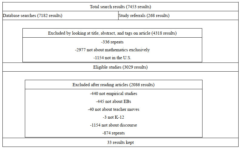
Assessment data, studies of opportunity-to-learn, and the extant beliefs of some U.S. teachers about the roles and abilities of emergent bilingual students make it necessary to consider how to improve mathematics instruction. This systematic, qualitative review of 33 studies in K-12 settings used a definition of discourse informed by systemic functional linguistics and positioning theory to answer the following question: How, if at all, does the literature suggest teachers encourage emergent bilingual students' participation in mathematics discourse and discourse communities through reflexive and interactive positioning? A coding process uncovered themes from the articles, all identified through methodical elimination and published in the last 25 years. Findings suggest that teachers can position students to partake in mathematics discourse by engaging in practices that reflect these students' abilities and strategies and show the value of their current communicative practices and out-of-school contexts.
- mathematics discourse,
- discourse community,
- emergent bilingual,
- positioning theory,
- revoicing,
- nonlinguistic resources
Citation: Kanushri Wadhwa. Facilitating emergent bilingual students' participation in mathematics discourse and discourse communities through positioning[J]. STEM Education, 2025, 5(2): 291-309. doi: 10.3934/steme.2025015

Related Papers:

Abstract

Assessment data, studies of opportunity-to-learn, and the extant beliefs of some U.S. teachers about the roles and abilities of emergent bilingual students make it necessary to consider how to improve mathematics instruction. This systematic, qualitative review of 33 studies in K-12 settings used a definition of discourse informed by systemic functional linguistics and positioning theory to answer the following question: How, if at all, does the literature suggest teachers encourage emergent bilingual students' participation in mathematics discourse and discourse communities through reflexive and interactive positioning? A coding process uncovered themes from the articles, all identified through methodical elimination and published in the last 25 years. Findings suggest that teachers can position students to partake in mathematics discourse by engaging in practices that reflect these students' abilities and strategies and show the value of their current communicative practices and out-of-school contexts.

References

[1]	Kaje, E.S., More than just good teaching: Teachers engaging culturally and linguistically diverse learners with content and language in mainstream classrooms. Doctoral dissertation, University of Washington, 2009, 1‒191.
[2]	García, O. and Kleifgen, J., Introduction, in Educating emergent bilinguals: Policies, programs, and practices for English language learners (Eds. Author 1 and Author 2), 2010, Teachers College Press.
[3]	Brenner, M., Development of mathematical communication in problem solving groups by language minority students. Bilingual Research Journal, 1998, 22(2/3/4): 103–128. https://doi.org/10.1080/15235882.1998.10162720 doi: 10.1080/15235882.1998.10162720
[4]	Willey, C., A case study of two teachers attempting to create active mathematics discourse communities with Latinos. Unpublished doctoral dissertation. University of Illinois, 2013, 1‒166.
[5]	National Center for Education Statistics. National assessment of educational progress 2019, 2019. Available from: https://www.nationsreportcard.gov/mathematics/nation/achievement/?grade = 4
[6]	Aguirre-Muñoz, Z. and Boscardin, C., Opportunity to learn and English learner achievement: Is increased content exposure beneficial? Journal of Latinos and Education, 2008, 7(3): 186‒205. https://doi.org/10.1080/15348430802100089 doi: 10.1080/15348430802100089
[7]	Bailey, A., Blackstock-Bernstein, A. and Heritage, M., At the intersection of mathematics and language: Examining mathematical strategies and explanations by grade and English learner status. The Journal of Mathematical Behavior, 2015, 40: 6‒28. https://doi.org/10.1016/j.jmathb.2015.03.007 doi: 10.1016/j.jmathb.2015.03.007
[8]	Aguirre-Muñoz, Z. and Amabisca, A., Defining opportunity to learn for English language learners: Linguistic and cultural dimensions of ELLs' instructional contexts. Journal of Education for Students Placed at Risk, 2010, 15(3): 259‒278. https://doi.org/10.1080/10824669.2010.495691 doi: 10.1080/10824669.2010.495691
[9]	de Araujo, Z., Roberts, S., Willey, C., and Zahner, W., English learners in K–12 mathematics education: A Review of the literature. Review of Educational Research, 2018, 88(6): 879‒919. https://doi.org/10.3102/0034654318798093 doi: 10.3102/0034654318798093
[10]	Drageset, O.G. and Ell, F., Using positioning theory to think about mathematics classroom talk. Educational Studies in Mathematics, 2023,115(1): 353‒385. https://doi.org/10.1007/s10649-023-10295-0 doi: 10.1007/s10649-023-10295-0
[11]	Schleppegrell, M., The Linguistic challenges of mathematics teaching and learning: A research review. Reading & Writing Quarterly: Overcoming Learning Difficulties, 2007, 23(2): 139‒159. http://dx.doi.org/10.1080/10573560601158461 doi: 10.1080/10573560601158461
[12]	Walshaw, M. and Anthony, G., The Teacher's role in classroom discourse: A review of recent literature into mathematics classrooms. Review of Educational Research, 2017, 78(3): 516‒551. https://doi.org/10.3102/0034654308320292 doi: 10.3102/0034654308320292
[13]	Smith, E.M., Facilitating emergent bilinguals' participation in mathematics: An examination of a teacher's positioning acts. Unpublished doctoral dissertation. University of Missouri, 2018, 1‒166.
[14]	Celedón-Pattichis, S., Peters, S., Borden, L., Males, J., Pape, S., Chapman, O., et al., Asset-based approaches to equitable mathematics education research and practice. Journal for Research in Mathematics Education, 2018, 49(4): 373‒389. https://doi.org/10.5951/jresematheduc.49.4.0373 doi: 10.5951/jresematheduc.49.4.0373
[15]	Gee, J., Social Linguistics and Literacies: Ideology in Discourses. Falmer Press, 1996.
[16]	Halliday, M.A.K., Language as social semiotic: The Social interpretation of languages and meaning. Hodder & Stoughton Educational, 1976.
[17]	Wenger, E., Communities of practice: Learning, meaning, and identity. Cambridge University Press, 1998.
[18]	Wagner, D. and Herbel-Eisenmann, B., Re-mythologizing mathematics through attention to classroom positioning. Educational Studies in Mathematics, 2009, 72(1): 1‒15. https://doi.org/10.1007/s10649-008-9178-5 doi: 10.1007/s10649-008-9178-5
[19]	Khisty, L.L. and Chval, K.B., Pedagogic discourse and equity in mathematics: When teachers' talk matters. Mathematics Education Research Journal, 2002, 14(3): 154–168. https://doi.org/10.1007/BF03217360 doi: 10.1007/BF03217360
[20]	Celedón-Pattichis, S., Kussainova, G., López-Leiva, C.A. and Pattichis, M.S., "Fake it until you make it": Participation and positioning of a Bilingual Latina student in mathematics and computing. Teachers College Record, 2022,124(5): 3‒228. https://doi.org/10.1177/01614681221103929 doi: 10.1177/01614681221103929
[21]	Banse, H., Palacios, N., Merritt, E. and Rimm-Kaufman, S., Scaffolding English language learners' mathematical talk in the context of Calendar Math. The Journal of Educational Research, 2017,110(2): 199‒208. http://dx.doi.org/10.1080/00220671.2015.1075187 doi: 10.1080/00220671.2015.1075187
[22]	Celedón-Pattichis, S. and Turner, E., "Explicame tu respuesta": Supporting the development of mathematical discourse in emergent bilingual kindergarten students. Bilingual Research Journal: The Journal of the National Association for Bilingual Education, 2012, 35(2): 197–216. https://doi.org/10.1080/15235882.2012.703635 doi: 10.1080/15235882.2012.703635
[23]	Chval, K., Pinnow, R. and Thomas, A., Learning how to focus on language while teaching mathematics to English language learners: A case study of Courtney. Mathematics Education Research Journal, 2014, 27(1): 103–127. https://doi.org/10.1007/s13394-013-0101-8 doi: 10.1007/s13394-013-0101-8
[24]	Dominguez, H., Bilingual students' articulation and gesticulation of mathematical knowledge during problem solving. Bilingual Research Journal, 2005, 29(2): 269–293. https://doi.org/10.1080/15235882.2005.10162836 doi: 10.1080/15235882.2005.10162836
[25]	Dominguez, H., Using what matters to students in bilingual mathematics problems, Educational Studies in Mathematics, 2011, 76(1): 305‒328. https://doi.org/10.1007/s10649-010-9284-z doi: 10.1007/s10649-010-9284-z
[26]	Dominguez, H., Lopez-Leiva, C. and Khisty, L., Relational engagement: Proportional reasoning with bilingual Latino/a students. Educational Studies in Mathematics, 2014, 85(1): 143‒160. https://doi.org/10.1007/S10649-013-9501-7 doi: 10.1007/S10649-013-9501-7
[27]	Dominguez, H., Social risk takers: understanding bilingualism in mathematical discussions. Issues in Teacher Education, 2017, 26(2): 35‒47.
[28]	Enyedy, N., Rubel, L., Castellón, V., Mukhopadhyay, S., Esmonde, I. and Secada, W., Revoicing in a multilingual classroom. Mathematical Thinking and Learning, 2008, 10(2): 134–162. https://doi.org/10.1080/10986060701854458 doi: 10.1080/10986060701854458
[29]	Hansen-Thomas, H., Learning to use math discourse in a standards-based, reform-oriented middle school classroom: How Latino/a ELLs becomes socialized into the math community of practice. Unpublished doctoral dissertation. University of Texas at San Antonio, 2005.
[30]	Hansen-Thomas, H., Reform-oriented mathematics in three 6th grade classes: How teachers draw in ELLs to academic discourse. Journal of Language, Identity and Education, 2009, 8(2-3): 88‒106. https://doi.org/10.1080/15348450902848411 doi: 10.1080/15348450902848411
[31]	Hufferd-Ackles, K., Fuson, K. and Sherin, M., Describing levels and components of a math-talk learning community. Journal for Research in Mathematics Education, 2004, 35(2): 81‒116. https://doi.org/10.2307/30034933 doi: 10.2307/30034933
[32]	McGraw, R. and Rubinstein-Ávila, E., Middle school immigrant students developing mathematical reasoning in Spanish and English. Bilingual Research Journal, 2008, 31(1-2): 147‒173. https://doi.org/10.1080/15235880802640656 doi: 10.1080/15235880802640656
[33]	Merritt, E., Palacios, N., Banse, H., Rimm-Kaufman, S. and Leis, M., Teaching practices in Grade 5 mathematics class with high-achieving English learner students. The Journal of Education Research, 2014,110(1): 17‒31. https://doi.org/10.1080/00220671.2015.1034352 doi: 10.1080/00220671.2015.1034352
[34]	Moschkovich, J., Academic literacy in mathematics for English Learners. The Journal of Mathematical Behavior, 2015, 40(A): 43–62. https://doi.org/10.1016/j.jmathb.2015.01.005 doi: 10.1016/j.jmathb.2015.01.005
[35]	Musanti, S. and Celedón-Pattichis, S., Promising pedagogical practices for emergent bilinguals in kindergarten: Towards a mathematics discourse community. Journal of Multilingual Education Research, 2013, 4(1): 41‒62.
[36]	Musanti, S.I., Celedón-Pattichis, S. and Marshall, M.E., Reflections on language and mathematics problem-solving: A Study of a bilingual first grade teacher. Bilingual Research Journal, 2009, 32(1): 25‒41.https://doi.org/10.1080/15235880902965763 doi: 10.1080/15235880902965763
[37]	Petkova, M., Classroom discourse and teacher talk influences on English language learner students' mathematics experience. Doctoral dissertation, University of South Florida. Proquest, 2009.
[38]	Rubinstein-Ávila, E., Sox, A.A., Kaplan, S. and McGraw, R., Does biliteracy + mathematical discourse = binumerate development? Language use in a middle-school dual-language mathematics classroom? Urban Education, 2014, 50(8): 899‒937. https://doi.org/10.1177/0042085914536997 doi: 10.1177/0042085914536997
[39]	Shein, P., Seeing with two eyes: A Teacher's use of gestures in questioning and revoicing to engage English language learners in the repair of mathematical errors. Journal for Research in Mathematics Education, 2012, 43(2): 182–222. https://doi.org/10.5951/jresematheduc.43.2.0182 doi: 10.5951/jresematheduc.43.2.0182
[40]	Smith, E., Facilitating emergent bilinguals' participation in mathematics: An examination of a teacher's positioning acts. Electronic Journal for Research in Science and Mathematics Education, 2023, 27(4): 77‒106.
[41]	Turner, E. and Celedón-Pattichis, S., Mathematical problem solving among Latina/o kindergarteners: An Analysis of opportunities to learn. Journal of Latinos and Education, 2011, 10(2): 146‒169. https://doi.org/10.1080/15348431.2011556524 doi: 10.1080/15348431.2011556524
[42]	Turner, E., Dominguez, H., Empson, S. and Maldonado, L., Latino/a bilinguals and their teachers developing a shared communicative space. Educational Studies in Mathematics, 2013, 84(1): 349‒370. https://doi.org/10.1007/s10649-013-9486 doi: 10.1007/s10649-013-9486
[43]	Turner, E., Dominguez, H., Maldonado, L., and Empson, S., English learners' participation in mathematical discussion: Shifting positionings and dynamic identities. Journal for Research in Mathematics Education, 2013, 44(1): 199–234. https://doi.org/10.5951/jresematheduc.44.1.0199 doi: 10.5951/jresematheduc.44.1.0199
[44]	Yang, J., Ozbek, G., Liang, S. and Cho, S., Effective teaching strategies for teaching mathematics to young gifted English learners. Gifted Education International, 2023, 39(2): 226‒246. https://doi.org/10.1177/02614294231165121 doi: 10.1177/02614294231165121
[45]	Zahner, W., How to do math with words: Learning algebra through peer discussions. Unpublished doctoral dissertation. University of California, 2011.
[46]	Zahner, W., The rise and run of a computational understanding of slope in a conceptually focused bilingual algebra class. Educational Studies in Mathematics, 2015, 88(1): 19–41. https://doi.org/10.1007/s10649-014-9575-x doi: 10.1007/s10649-014-9575-x
[47]	Zahner, W., Calleros, E.D. and Pelaez, K., Designing learning environments to promote academic literacy in mathematics in multilingual secondary mathematics classrooms. ZDM- Mathematics Education, 2021, 53(1): 359‒373. https://doi.org/10.1007/s11858-021-01239-0 doi: 10.1007/s11858-021-01239-0
[48]	Zahner, W., Velazquez, G., Moschkovich, J., Vahey, P. and Lara-Meloy, T., Mathematics teacher practices with technology that support conceptual understanding for Latino/a students. The Journal of Mathematical Behavior, 2012, 31(4): 431‒446. https://doi.org/10.1016/j.jmathb.2012.06.002 doi: 10.1016/j.jmathb.2012.06.002
[49]	Echevarria, J. and Short, D., Programs and practices for effective sheltered content instruction in Improving Education for English Learners: Research-Based Approaches (eds. Author 1 and Author 2), CDE Press, 2010.
[50]	Wadhwa, K., Positioning emergent bilingual and racially minoritized students to participate in mathematics discourse and discourse communities, Unpublished doctoral dissertation, University of Miami, 2023.

Author's biography Dr. Kanushri Wadhwa is a mathematics teacher in the New York City Department of Education. Her research interests include equity in mathematics classrooms and teachers' experiences in bridging research and practice

Reader Comments

Your name:*

Email:*
© 2025 the Author(s), licensee AIMS Press. This is an open access article distributed under the terms of the Creative Commons Attribution License (http://creativecommons.org/licenses/by/4.0)