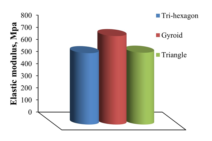
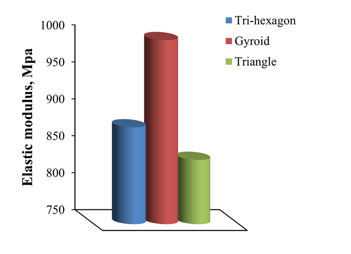
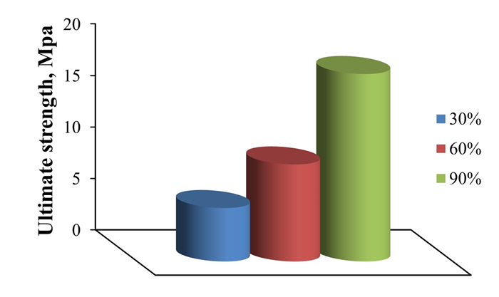
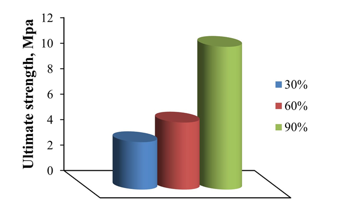
This paper studied the mechanical properties of carbon fiber-reinforced polylactic acid (CF-PLA) samples manufactured with three different 3D-printed patterns: gyroid, tri-hexagon, and triangular. Filler content was generated in the samples at infill ratios of 30%, 60%, and 90%. Conventional tensile, flexural, impact, and fatigue tests were conducted to investigate the mechanical properties. It was found that the gyroid infill pattern enhanced performance, exhibiting tensile strength and modulus of elasticity up to 63% and 13% greater, respectively, than the tri-hexagon pattern at a 90% infill ratio. The fatigue life improvement was 113% compared with the tri-hexagon pattern. The tensile strength and modulus of elasticity increased up to 35% and 40% after including carbon fibers. The increase in flexural modulus was 30% compared to the triangular pattern, whereas impact energy absorption reached the best result with the triangular pattern, up to 89% more than the gyroid pattern. These results elucidate the optimization of infill patterns and ratios together with carbon fiber reinforcement for the development of CF-PLA components as a high-performance 3D printing solution for a wide range of engineering applications.
Citation: Lubna Layth Dawood, Ehsan Sabah AlAmeen. Influence of infill patterns and densities on the fatigue performance and fracture behavior of 3D-printed carbon fiber-reinforced PLA composites[J]. AIMS Materials Science, 2024, 11(5): 833-857. doi: 10.3934/matersci.2024041
This paper studied the mechanical properties of carbon fiber-reinforced polylactic acid (CF-PLA) samples manufactured with three different 3D-printed patterns: gyroid, tri-hexagon, and triangular. Filler content was generated in the samples at infill ratios of 30%, 60%, and 90%. Conventional tensile, flexural, impact, and fatigue tests were conducted to investigate the mechanical properties. It was found that the gyroid infill pattern enhanced performance, exhibiting tensile strength and modulus of elasticity up to 63% and 13% greater, respectively, than the tri-hexagon pattern at a 90% infill ratio. The fatigue life improvement was 113% compared with the tri-hexagon pattern. The tensile strength and modulus of elasticity increased up to 35% and 40% after including carbon fibers. The increase in flexural modulus was 30% compared to the triangular pattern, whereas impact energy absorption reached the best result with the triangular pattern, up to 89% more than the gyroid pattern. These results elucidate the optimization of infill patterns and ratios together with carbon fiber reinforcement for the development of CF-PLA components as a high-performance 3D printing solution for a wide range of engineering applications.

| [1] |
Ayatollahi MR, Nabavi-Kivi A, Bahrami B, et al. (2020) The influence of in-plane raster angle on tensile and fracture strengths of 3D-printed PLA specimens. Eng Fract Mech 237: 107225. https://doi.org/10.1016/j.engfracmech.2020.107225 doi: 10.1016/j.engfracmech.2020.107225

|
| [2] |
Ogaili AAF, Basem A, Kadhim MS, et al. (2024) The effect of chopped carbon fibers on the mechanical properties and fracture toughness of 3D-printed PLA parts: An experimental and simulation study. J Compos Sci 8: 273. https://doi.org/10.3390/jcs8070273 doi: 10.3390/jcs8070273
|
| [3] |
Vălean E, Foti P, Razavi SMJ, et al. (2023) Static and fatigue behavior of 3D printed PLA and PLA reinforced with short carbon fibers. J Mech Sci Technol 37: 5555–5559. https://doi.org/10.1007/s12206-023-0822-2 doi: 10.1007/s12206-023-0822-2
|
| [4] |
Ogaili AAF, Jaber AA, Hamzah MN (2023) Wind turbine blades fault diagnosis based on vibration dataset analysis. Data Brief 49: 109414. https://doi.org/10.1016/j.dib.2023.109414 doi: 10.1016/j.dib.2023.109414
|
| [5] |
Simmons H, Tiwary P, Colwell JE, et al. (2019) Improvements in the crystallinity and mechanical properties of PLA by nucleation and annealing. Polym Degrad Stab 166: 248–257. https://doi.org/10.1016/j.polymdegradstab.2019.05.036 doi: 10.1016/j.polymdegradstab.2019.05.036
|
| [6] | Kumar Patro P, Kandregula S, Suhail Khan MN, et al. (2023) Investigation of mechanical properties of 3D printed sandwich structures using PLA and ABS. Mater Today Proc. https://doi.org/10.1016/j.matpr.2023.08.366 |
| [7] |
Ogaili AAF, Jaber AA, Hamzah MN (2023) A methodological approach for detecting multiple faults in wind turbine blades based on vibration signals and machine learning. Curved Layer Struct 10: 20220214. https://doi.org/10.1515/cls-2022-0214 doi: 10.1515/cls-2022-0214
|
| [8] |
Jap NSF, Pearce GM, Hellier AK, et al. (2019) The effect of raster orientation on the static and fatigue properties of filament deposited ABS polymer. Int J Fatigue 124: 328–337. https://doi.org/10.1016/j.ijfatigue.2019.03.018 doi: 10.1016/j.ijfatigue.2019.03.018
|
| [9] |
Dizon JRC, Espera AH, Chen Q, et al. (2018) Mechanical characterization of 3D-printed polymers. Addit Manuf 20: 44–67. https://doi.org/10.1016/j.addma.2017.12.002 doi: 10.1016/j.addma.2017.12.002
|
| [10] |
Popescu D, Zapciu A, Amza C, et al. (2018) FDM process parameters influence over the mechanical properties of polymer specimens: A review. Polym Test 69: 157–166. https://doi.org/10.1016/j.polymertesting.2018.05.020 doi: 10.1016/j.polymertesting.2018.05.020
|
| [11] |
Chacón JM, Caminero MA, García-Plaza E, et al. (2017) Additive manufacturing of PLA structures using fused deposition modelling: Effect of process parameters on mechanical properties and their optimal selection. Mater Design 124: 143–157. https://doi.org/10.1016/j.matdes.2017.03.065 doi: 10.1016/j.matdes.2017.03.065
|
| [12] | Rezanezhad S, Azadi M (2024) The influence of 3D-printed PLA coatings on pure and fretting fatigue properties of AM60 magnesium alloys under cyclic bending loads. Heliyon 10: e29552. https://doi.org/10.1016/j.heliyon.2024.e29552 |
| [13] |
Rodríguez-Panes A, Claver J, Camacho AM (2018) The influence of manufacturing parameters on the mechanical behaviour of PLA and ABS pieces manufactured by FDM: A comparative analysis. Materials 11: 1333. https://doi.org/10.3390/ma11081333 doi: 10.3390/ma11081333
|
| [14] |
Tymrak BM, Kreiger M, Pearce JM (2014) Mechanical properties of components fabricated with open-source 3-D printers under realistic environmental conditions. Mater Design 58: 242–246. https://doi.org/10.1016/j.matdes.2014.02.038 doi: 10.1016/j.matdes.2014.02.038
|
| [15] |
Sajjadi SA, Ashenai Ghasemi F, Rajaee P, et al. (2022) Evaluation of fracture properties of 3D printed high impact polystyrene according to essential work of fracture: Effect of raster angle. Addit Manuf 59: 103191. https://doi.org/10.1016/j.addma.2022.103191 doi: 10.1016/j.addma.2022.103191
|
| [16] |
Karimi HR, Khedri E, Nazemzadeh N, et al. (2023) Effect of layer angle and ambient temperature on the mechanical and fracture characteristics of unidirectional 3D printed PLA material. Mater Today Commun 35: 106174. https://doi.org/10.1016/j.mtcomm.2023.106174 doi: 10.1016/j.mtcomm.2023.106174
|
| [17] |
Ganeshkumar S, Kumar SD, Magarajan U, et al. (2022) Investigation of tensile properties of different infill pattern structures of 3D-printed PLA polymers: Analysis and validation using finite element analysis in ANSYS. Materials 15: 5142. https://doi.org/10.3390/ma15155142 doi: 10.3390/ma15155142
|
| [18] |
Srinivasan R, Ruban W, Deepanraj A, et al. (2020) Effect on infill density on mechanical properties of PETG part fabricated by fused deposition modelling. Mater Today Proc 27: 1838–1842. https://doi.org/10.1016/j.matpr.2020.03.788 doi: 10.1016/j.matpr.2020.03.788
|
| [19] |
Casavola C, Cazzato A, Moramarco V, et al. (2016) Orthotropic mechanical properties of fused deposition modelling parts described by classical laminate theory. Mater Design 90: 453–458. https://doi.org/10.1016/j.matdes.2015.11.009 doi: 10.1016/j.matdes.2015.11.009
|
| [20] |
Domingo-Espin M, Puigoriol-Forcada JM, Garcia-Granada AA, et al. (2015) Mechanical property characterization and simulation of fused deposition modeling Polycarbonate parts. Mater Design 83: 670–677. https://doi.org/10.1016/j.matdes.2015.06.074 doi: 10.1016/j.matdes.2015.06.074
|
| [21] |
Lanzotti A, Grasso M, Staiano G, et al. (2015) The impact of process parameters on mechanical properties of parts fabricated in PLA with an open-source 3-D printer. Rapid Prototyping J 21: 604–617. https://doi.org/10.1108/RPJ-09-2014-0135 doi: 10.1108/RPJ-09-2014-0135
|
| [22] |
Gurrala PK, Regalla SP (2014) Part strength evolution with bonding between filaments in fused deposition modelling: This paper studies how coalescence of filaments contributes to the strength of final FDM part. Virtual Phys Prototy 9: 141–149. https://doi.org/10.1080/17452759.2014.913400 doi: 10.1080/17452759.2014.913400
|
| [23] |
Gomez-Gras G, Jerez-Mesa R, Travieso-Rodriguez JA, et al. (2018) Fatigue performance of fused filament fabrication PLA specimens. Mater Design 140: 278–285. https://doi.org/10.1016/j.matdes.2017.11.072 doi: 10.1016/j.matdes.2017.11.072
|
| [24] |
Hu Y, Lin Y, Yang L, et al. (2024) Additive manufacturing of carbon fiber-reinforced composites: A review. Appl Compos Mater 31: 353–398. https://doi.org/10.1007/s10443-023-10211-0 doi: 10.1007/s10443-023-10211-0
|
| [25] |
Ogaili AAF, Al-Ameen ES, Kadhim MS, et al. (2020) Evaluation of mechanical and electrical properties of GFRP composite strengthened with hybrid nanomaterial fillers. AIMS Mater Sci 7: 93–102. https://doi.org/10.3934/matersci.2020.1.93 doi: 10.3934/matersci.2020.1.93
|
| [26] | Al-Ameen ES, Al-Sabbagh MNM, Ogaili AAF, et al. (2022) Role of pre-stressing on anti-penetration properties for kevlar/epoxy composite plates. Int J Nanoelectron Mater 15: 293–302. Available from: http://www.ijneam.unimap.edu.my/images/PDF/Vol15No4/IJNEAM-V15N4P1.pdf. |
| [27] |
Ogaili AAF, Hamzah MN (2022) Integration of machine learning (ML) and finite element analysis (FEA) for predicting the failure modes of a small horizontal composite blade. IJRER 4: 2168–2179. https://doi.org/10.20508/ijrer.v12i4.13354.g8589 doi: 10.20508/ijrer.v12i4.13354.g8589
|
| [28] |
Hamdan ZK, Ogaili AAF, Metteb ZW, et al. (2021) Study the electrical, thermal behaviour of (glass/jute) fibre hybrid composite material. J Phys Conf Ser 1783: 012070. https://doi.org/10.1088/1742-6596/1879/1/012070 doi: 10.1088/1742-6596/1879/1/012070
|
| [29] |
Abdulla FA, Qasim MS, Ogaili AAF (2021) Influence eggshells powder additive on thermal stress of fiberglass/polyester composite tubes. IOP Conf Ser Earth Environ Sci 877: 012039. https://doi.org/10.1088/1755-1315/779/1/012039 doi: 10.1088/1755-1315/779/1/012039
|
| [30] |
Ogaili AAF, Abdulla FA, Al-Sabbagh MNM, et al. (2020) Prediction of mechanical, thermal and electrical properties of wool/glass fiber based hybrid composites. IOP Conf Ser Mater Sci Eng 928: 022004. https://doi.org/10.1088/1757-899X/870/1/022004 doi: 10.1088/1757-899X/870/1/022004
|
| [31] | Mohammed KA, Al-Sabbagh MNM, Ogaili AAF, et al. (2020) Experimental analysis of hot machining parameters in surface finishing of crankshaft. JMERD 43: 105–114. |
| [32] |
Cao M, Cui T, Yue Y, et al. (2023) Preparation and characterization for the thermal stability and mechanical property of PLA and PLA/CF samples built by FFF approach. Materials 16: 5023. https://doi.org/10.3390/ma16145023 doi: 10.3390/ma16145023
|
| [33] |
Monaldo E, Ricci M, Marfia S (2023) Mechanical properties of 3D printed polylactic acid elements: Experimental and numerical insights. Mech Mater 177: 104551. https://doi.org/10.1016/j.mechmat.2023.104551 doi: 10.1016/j.mechmat.2023.104551
|
| [34] |
Ivey M, Melenka GW, Carey JP, et al. (2017) Characterizing short-fiber-reinforced composites produced using additive manufacturing. Adv Manuf-Polym Comp 3: 81–91. https://doi.org/10.1080/20550340.2017.1341125 doi: 10.1080/20550340.2017.1341125
|
| [35] |
Tian X, Liu T, Yang C, et al. (2016) Interface and performance of 3D printed continuous carbon fiber reinforced PLA composites. Composites Part A 88: 198–205. https://doi.org/10.1016/j.compositesa.2016.05.032 doi: 10.1016/j.compositesa.2016.05.032
|
| [36] |
Zhang H, Yang D, Sheng Y (2018) Performance-driven 3D printing of continuous curved carbon fibre reinforced polymer composites: A preliminary numerical study. Compos Part B-Eng 151: 256–264. https://doi.org/10.1016/j.compositesb.2018.06.017 doi: 10.1016/j.compositesb.2018.06.017
|
| [37] |
Wang X, Jiang M, Zhou Z, et al. (2017) 3D printing of polymer matrix composites: A review and prospective. Compos Part B-Eng 110: 442–458. https://doi.org/10.1016/j.compositesb.2016.11.034 doi: 10.1016/j.compositesb.2016.11.034
|
| [38] |
Yang L, Zhou L, Lin Y, et al. (2024) Failure mode analysis and prediction model of additively manufactured continuous carbon fiber-reinforced polylactic acid. Polym Compos 45: 7205–7221. https://doi.org/10.1002/pc.28261 doi: 10.1002/pc.28261
|
| [39] |
Dogru A, Sozen A, Neser G, et al. (2021) Effects of aging and infill pattern on mechanical properties of hemp reinforced PLA composite produced by fused filament fabrication (FFF). ASEP 14: 651–660. https://doi.org/10.14416/j.asep.2021.08.007 doi: 10.14416/j.asep.2021.08.007
|
| [40] |
Kumar KR, Mohanavel V, Kiran K (2022) Mechanical properties and characterization of polylactic acid/carbon fiber composite fabricated by fused deposition modeling. J Mater Eng Perform 31: 4877–4886. https://doi.org/10.1007/s11665-021-06566-7 doi: 10.1007/s11665-021-06566-7
|
| [41] |
Dong G, Tang Y, Zhao YF (2017) A survey of modeling of lattice structures fabricated by additive manufacturing. J Mech Design 139: 100906. https://doi.org/10.1115/1.4037305 doi: 10.1115/1.4037305
|
| [42] |
Li L, Liu W, Sun L (2022) Mechanical characterization of 3D printed continuous carbon fiber reinforced thermoplastic composites. Compos Sci Technol 227: 109618. https://doi.org/10.1016/j.compscitech.2022.109618 doi: 10.1016/j.compscitech.2022.109618
|
Figures(23) / Tables(5)

Lubna Layth Dawood, Ehsan Sabah AlAmeen. Influence of infill patterns and densities on the fatigue performance and fracture behavior of 3D-printed carbon fiber-reinforced PLA composites[J]. AIMS Materials Science, 2024, 11(5): 833-857. doi: 10.3934/matersci.2024041


 DownLoad: